The document discusses matrices and their applications in engineering mathematics. It presents five theorems regarding properties of matrices such as:
1) The eigenvectors of a matrix corresponding to distinct eigenvalues are orthogonal.
2) The characteristic polynomial of the adjoint of a matrix is equal to the characteristic polynomial of the original matrix with the eigenvalues replaced by their reciprocals.
3) The eigenvalues of an orthogonal matrix have absolute value of 1.
4) If the eigenvalue of an orthogonal matrix is not ±1, then the associated eigenvector is the zero vector.
5) The eigenvectors corresponding to distinct eigenvalues of a symmetric matrix are orthogonal.
It also provides examples of finding the eigenvalues and eigenvectors of specific matrices.
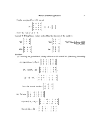
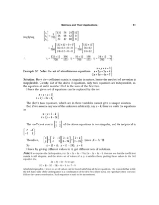
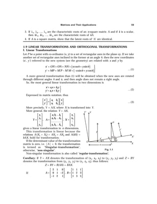
![Matrices and Their Applications 55
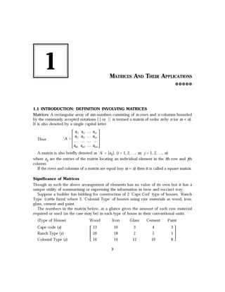
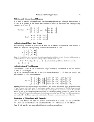
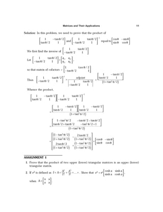
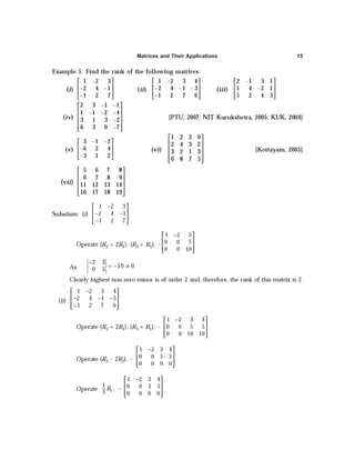
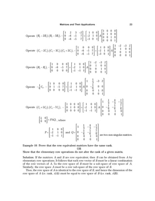
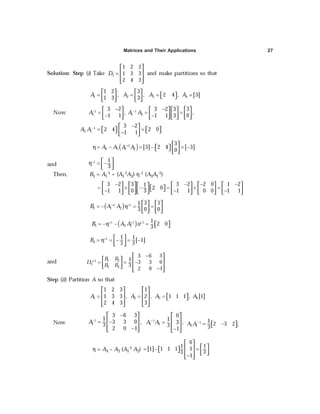
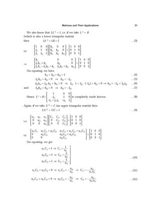
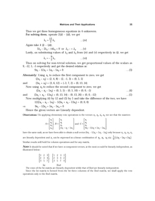
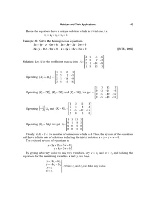
aAX1 + bAX2 + cAX3 = aλ1X1 + bλ2X2 + cλ3X3 = 0, as [A – λiI]Xi = 0 …(2)
Multiply (2) by A, again, and obtain
aλ1
2X1 + bλ2
2X2 + cλ3
2X3 = 0 …(3)
Now writing (1), (2), (3) together as
1
1 2 3 2
2 2 2
3
1 2 3
1 1 1
0
aX
bX
cX
λ λ λ =
λ λ λ
…(4)
Now we see that
( )( )( )
= λ λ λ = − λ − λ λ − λ λ − λ ≠
λ λ λ
1 2 3 1 2 2 3 3 1
2 2 2
1 2 3
1 1 1
| | 0
B
Hence B–1 exists.
Multiplying (4) by B–1 results in,
1
2
3
.
0
aX
bX
cX
=
But this requires a = b = c = 0 which is contrary to the hypothesis.
Thus X1, X2, X3 are linearly independent.
Theorem 2: If λ
λ
λ
λ
λ be a non-zero characteristic root (eigen value) of the non-singular n-
square matrix A, then
| |
A
λ
is a charactristic polynomial of adjoint A.
Proof: For non-singular n-square matrix A, the ‘characteristic polynomial’
φ(λ) = |λI – A| = λn + s1λn–1 + s2λn–2 + … + sn–1 λ1 + (–1)n |A| …(1)
where sr (r = 1, 2, …, n – 1) is (–1)r times the sum of all the r-square principal minors of A.
Corresponding characteristic equation is given by
λn + s1λn–1 + s2λn–2 + … + (–1)n |A| = 0 …(2)
and on the same lines
|µI – Adj · A|= µn + s1µn–1 + s2µn –2 + … + sn –1 µ + (–1)n|Adj · A| …(3)
where sr (r = 1, 2, …, n – 1) is (–1)r times the sum of the r-square principal minors of Adj ·A.
Thus by the property |adj A| = |A|n–1 and definition of sr
we have ( )
( )
−
−
−
= −
= −
= −
M
M
1 1
2 2,
1 1
( 1)
1
1 ;
n
n
n
n
n
n
s s
s A s
s A s
…(4)
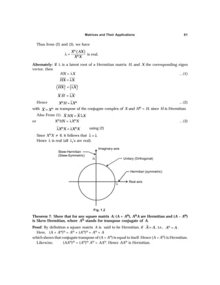
then |µI – adj · A| = (–1)n {(–1)n µn + sn–1 µn – 1 + sn– 2 µn–2 |A|
+ … + s2|A|n–3µ2 + s1|A|n–2µ + |A|n–1}](https://image.slidesharecdn.com/1-matricesandtheirapplications-231130153040-bda6e4b4/85/1-Matrices-and-their-Applications-pdf-53-320.jpg)
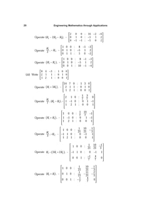
![Engineering Mathematics through Applications
56
( ) ( )
−
−
µ µ µ
= − + +…+ + − = µ
1
1 1
1 1 ( 1)
n n
n n
n
s s A f
A A A …(5)
Now
( ) ( ) ( ) ( ) ( )
1
1 1
1 1 1
1 1 1
n n
n n
n
A
f s s A
−
−
= − + +…+ + −
λ λ λ λ
…(6)
and by equation (2), we have
( ) ( )
{ }
1
1 1
1 1 0
n n
n n n
n
A
f s s A
−
−
λ = − λ + λ +…+ λ + − =
λ
Hence, A
λ
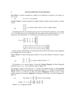
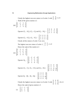
is a characteristic root of adjoint A.
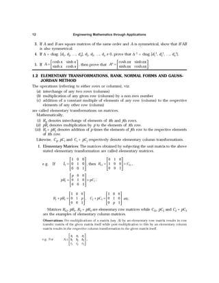
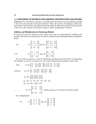
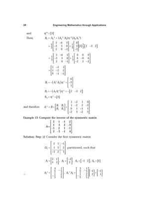
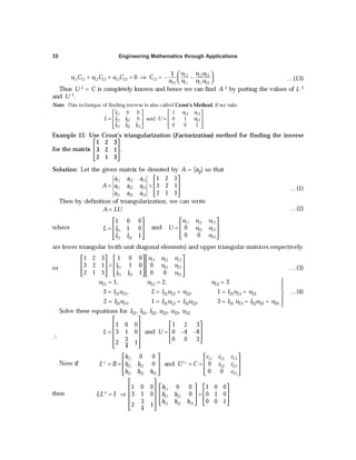
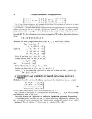
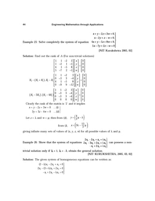
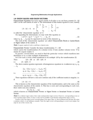
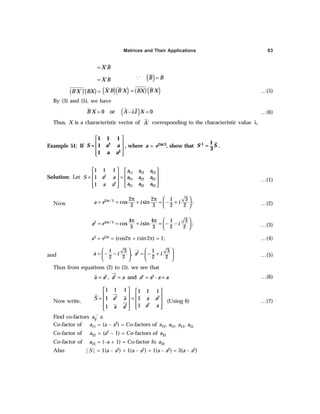
Theorem 3: Eigen values (characteristic roots) of orthogonal matrix A are of absolute value 1.
Proof: Let λi, Xi be characteristic roots and associated (characteristic vectors) invariant vectors
of an orthogonal matrix A, then
Xi´ Xi = X1
´ (A´ A) Xi = (AXi)´ (AXi), since for orthogonal A, A´A = I
⇒ Xi´ Xi = (λiXi)´ (λiXi) = (λi´Xc
´) (λiXi) = λiλi Xi´ Xi
or (1 – λiλi) Xi´Xi = 0 implies (1 – λiλi) = 0, since xi
´xi ≠ 0
Thus |λi| = 1.
Theorem 4: Prove if λ
λ
λ
λ
λi ≠
≠
≠
≠
≠ ± 1 is a characteristic root and Xi is the associated invariant vector
of an orthogonal matrix A, then Xi´ Xi = 0.
Proof: For characteristic value λi and corresponding characteristic vector Xi of the orthogonal
matrix A, we have
Xi´ Xi = Xi´ (A´ A) Xi = (AXi)´(AXi), (as A is given orthogonal)
⇒ Xi´Xi = (λiXi)´ (λiXi) = λiλiXi
´Xi, Using the transformation, AXi = λiXi
⇒ (1 – λiλi)Xi´ Xi = 0
⇒ Either (1 – λiλi) = 0 or Xi´ Xi = 0 But λi ≠ ±1
Hence Xi´Xi = 0.
Theorem 5: For a symmetrical square matrix, show that the eigen vectors corresponding to
two unequal eigen values are orthogonal. [NIT Kurukshetra, 2004; KUK, 2004, 2006 ]
Proof: Let A be any symmetric matrix i.e., A´ = A and λ1 and λ2 two unequal eigen values,
i.e., λ1 ≠ λ2
Let X1 and X2 be the two corresponding eigen vectors.
Now for λ1, (A – λ1I) X1 = 0](https://image.slidesharecdn.com/1-matricesandtheirapplications-231130153040-bda6e4b4/85/1-Matrices-and-their-Applications-pdf-54-320.jpg)
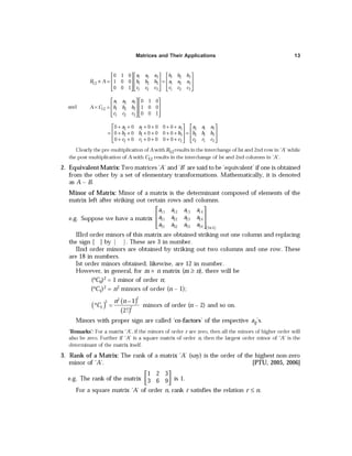
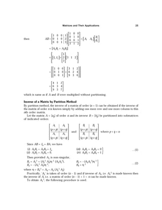
![Matrices and Their Applications 57
or AX1 = λ1X1 …(i)
Similarly AX2 = λ2X2 …(ii)
Taking the transpose of (ii), we get
(AX2)´ = (λ2X2)´
X2́A´ = λ2X2´ (as λ2 is an arbitrary constant)
X2
´A = λ2X2´ (Since A´ = A)
X2
´AX1 = λ2X2
´X1
X2
´ (λ1X1) = λ2X2
´X1 (As AX1 = λ1X1)
λ1X2
´X1 = λ2X2
´X1
(λ1 – λ2) X2́ X1 = 0 But λ1 – λ2 ≠ 0
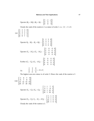
∴ X2́X1 = 0
If
=
1
1 2
3
x
X x
x
and
1
2 2
3
y
X y
y
=
∴
= = + +
1
2 1 1 2 3 2 1 1 2 2 3 3
3
´
x
X X y y y x y x y y y y
x
Clearly, (y1x1 + y2x2 + y3x3) = 0
This means, the two system of co-ordinates are orthogonal.
∴ Hence the transformation is an orthogonal transformation.
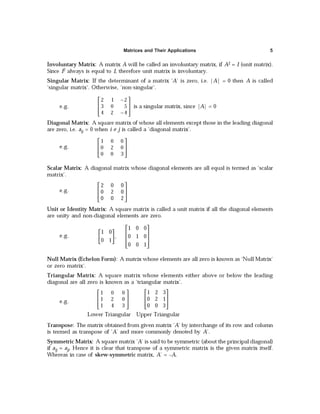
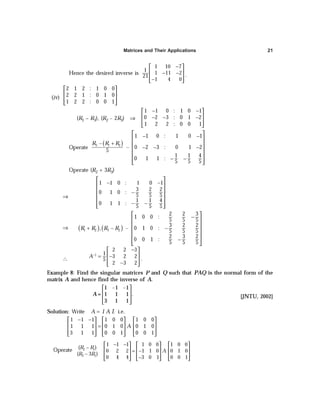
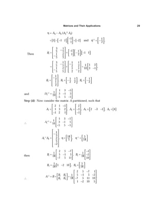
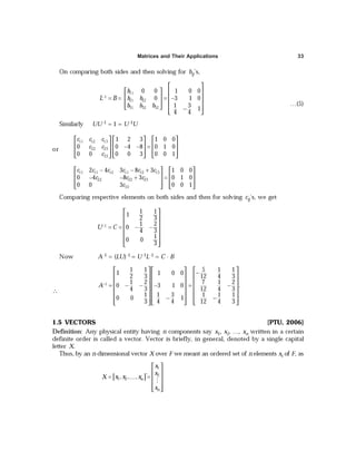
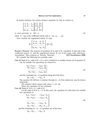
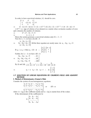
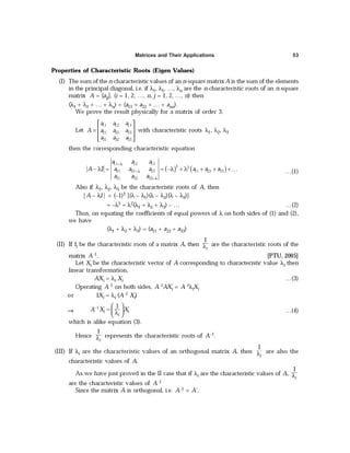
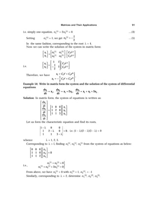
Example 33: Determine the eigen values and eigen vectors of
– 2 2 – 3
= 2 1 – 6
– 1 – 2 0
A
[NIT Kurukshetra, 2008]
Solution: The characteristic equation,
2 2 3
2 1 6 0
1 2
− − λ −
− λ − =
− − −λ
or λ3 + λ2 –21λ – 45 = 0
⇒ The roots of above equation are 5, –3, –3.
Putting λ = 5, the equations to be solved for x1, x2, x3 are [A – λI]x = 0
i.e. –7x + 2y – 3z = 0, 2x – 4y – 6z = 0, –x – 2y – 5z = 0.
Note that third equation is dependent on first two i.e. R1 + 2R2 ¾ R3
Solving them, we get x = k, y = 2k, z = –k
Similarly for λ = –3, the equations are
x + 2y – 3z = 0, 2x + 4y – 6z = 0, –x – 2y + 3z = 0
Second and third equations are derived from the first. Therefore, only one equation is
independent in this case.](https://image.slidesharecdn.com/1-matricesandtheirapplications-231130153040-bda6e4b4/85/1-Matrices-and-their-Applications-pdf-55-320.jpg)
![Engineering Mathematics through Applications
58
Taking z = 0, y = 1, we get x = –2. Again taking y = 0, z = 1, we get x = 3. Two linearly
independent eigen vectors are (–2, 1, 0) and (3, 0, 1). A linear combination of these viz.
(–2 + 3k, 1, k) is also an eigen vector.
Example 34: Find Eigen values and Eigen vectors for
6 –2 2
A = –2 3 –1 .
2 –1 3
Solution: The characteristic equation,
|A – λI| = 0 ⇒
− λ −
− − λ − =
− − λ
6 2 2
2 3 1 0
2 1 3
–λ3 + 12λ2 – 36λ + 32 = 0,
⇒ λ = 2, 2, 8 are the characteristic roots (latent roots).
Considering [A – 8I]X = 0, we may show that there exists only one linearly independent
solution
2
1
1
−
so that every non-zero multiple of the same is a characteristic vector for the characteristic
root 8.
For the characteristic root 2, we have
[A – 2I]X = 0 ⇒
4 2 2
2 1 1 0
2 1 1
x
y
z
−
− − =
−
or 4x – 2y + 2z = 0 …(i)
–2x + y – z = 0 …(ii)
2x – y + z = 0 …(iii)
which are equivalent to a single equation.
Thus we obtain two linearly independent solutions, may take as
1 1
0 and 2
2 0
−
The sub-space of V2 possessed by these two vectors is the characteristic space for the root 2.
ASSIGNMENT 2
1. The characteristic roots of A and A´ are the same.
2. The characteristic roots of A and ´
A are the conjugates of the characteristic roots of A.](https://image.slidesharecdn.com/1-matricesandtheirapplications-231130153040-bda6e4b4/85/1-Matrices-and-their-Applications-pdf-56-320.jpg)
![Matrices and Their Applications 61
or more precisely, Y = AX, where
cos sin
, and ,
sin cos
x
Y A X
y
α − α
ξ
= = =
α α
η
representing
linear transformation with A as the matrix of transformation.
Now,
cos sin
sin cos
A'
α α
=
− α α
…(3)
Find,
cos sin cos sin 1 0
´ 1
sin cos sin cos 0 1
AA
α − α α α
= = =
α α − α α
Also A'A = I. Hence A is an orthogonal matrix.
But if A is an orthogonal, then A' = A–1.
Thus, for the transformation Y = AX, we can write the inverse transformation
X = A–1Y, where 1 cos sin
´
sin cos
A A
− α α
= =
− α α
.
Example 36: Is the matrix
2 – 3 1
4 3 1
– 3 1 9
orthogonal? If not, can it be converted into an
orthogonal matrix? [KUK, 2005]
Solution: Let the given matrix be A. Then to check its orthogonality, find AA'
Thus
2 3 1 2 4 3
´ 4 3 1 3 3 1
3 1 9 1 1 9
AA
− −
= −
−
=
4 9 1 8 9 1 6 3 9 14 0 0
8 9 1 16 9 1 12 3 9 0 26 0
6 3 9 12 3 9 9 1 81 0 0 91
+ + − + − − +
− + + + − + + =
− − + − + + + +
As AA' ≠ I, hence A is not an orthogonal matrix.
However, it can be made an orthogonal by nromalization, i.e. on dividing every element
of a row by the square root of the sum of squares of each element of the respective row so
that product of resultant matrix (normalization) with its transpose would be a unit matrix.
Hence, the orthogonal form of the matrix A is
2 3 1
14 14 14
4 3 1
.
26 26 26
3 1 9
91 91 91
−
−
](https://image.slidesharecdn.com/1-matricesandtheirapplications-231130153040-bda6e4b4/85/1-Matrices-and-their-Applications-pdf-59-320.jpg)
![Matrices and Their Applications 63
Theorem 1: Prove that both ‘the inverse and transpose’ of an orthogonal matrix are also
orthogonal.
Solution: As we know that for an orthogonal matrix say A,
AA' = I = A'A and A' = A–1
Let A–1 = B
Case I: Then for B to be an orthogonal, we are to prove that
BB' = B'B = I
∴ BB' = (A–1) (A–1)´ = A–1(A')–1 = A–1(A–1)–1 = A–1A = I
Similarly, B'B = (A–1)' A–1 = (A')–1A–1 = (A–1)–1A–1 = AA–1 = I
Hence inverse of an orthogonal matrix is also an orthogonal.
Case II: Let A' = B. For B to be orthogonal, we need to prove that
BB´ = I = B´B
∴ BB´ = A'(A')' = A'A = I;
Also B'B = (A')'A' = AA' = I
Hence transpose of an orthogonal matrix is also orthogonal.
Theorem 2: A linear transformation preserves length if and only if its matrix is orthogonal.
Solution: Let Y1, Y2 be the respective images of X1, X2 under the linear transformation
Y = AX
Suppose A is orthogonal, then AA' = I = A'A
Now,
Y1 · Y2 = Y1
'Y2 = (AX1)'(AX2) = X1´ (A´A)X2 = X1 · X2 inner product.
Hence the transformation preserves length.
For vice versa, suppose lengths (i.e., inner products) are preserved.
Then, Y1 · Y2 = Y1' Y2 = (AX1)´ (AX2) = X1´ (A´A) X2
But, Y1 · Y2 = X1 · X2 (given) i.e., X1´ (A´A)X2 must be equal to X1 · X2 which is only possible
when A´A = I
Hence A is orthogonal.
For example, the linear transformation
1 2 2
3 3 3
2 1 2
3 3 3
2 2 1
3 3 3
Y AX X
= = −
−
is orthogonal.
The image of X = [a b c]' is
2 2 2 2 2 2
3 3 3 3 3 3 3 3 3
a b c a b c a b c
Y
= + + + − − +
and both vectors are of length 2 2 2
a b c
+ + .](https://image.slidesharecdn.com/1-matricesandtheirapplications-231130153040-bda6e4b4/85/1-Matrices-and-their-Applications-pdf-61-320.jpg)
![Matrices and Their Applications 65
Solution: We know that for an orthogonal matrix A, AA´ = I = A´A and A´ = A–1
∴
1 1 1 1 2 3
2 2 2 1 2 3
3 3 3 1 2 3
´
l m n l l l
AA l m n m m m
l m n n n n
=
, for given A.
2 2 2
1 1 1 1 2 1 2 1 2 1 3 1 3 1 3
2 2 2
2 1 2 1 2 1 2 2 2 2 3 2 3 2 3
2 2 2
3 1 3 1 3 1 3 2 3 2 3 2 3 3 3
l m n l l m m n n l l m m n n
l l m m n n l m n l l m m n n
l l m m n n l l m m n n l m n
+ + + + + +
= + + + + + +
+ + + + + +
For A to be an orthogonal, AA´ = I which is possible only if,
(l1
2 + m1
2 + n1
2) = (l2
2 + m2
2 + n2
2) = (l3
2 + m3
2 + n3
2) = 1
and (l1l2 + m1m2 + n1n2) = (l2l3 + m2m3 + n2n3) = (l3l1 + m3m1 + n3n1) = 0.
ASSIGNMENT 3
1. Prove that the product of two orthogonal matrix is orthogonal.
2. Prove that the matrix
cos 0 sin
0 1 0
sin 0 cos
θ θ
− θ θ
is an orthogonal matrix.
3. Given that ,
a b c
A b c a
c a b
=
where a, b, c are the roots of x3 + x2 + k = 0
(where k is a constant). Prove that ‘A’ is orthogonal.
4. Show that the modulus of an orthogonal transformation is either 1 or –1.
[Hint: Since AA' = I, then |A||A'| = |1|]
1.10 DIAGONALISATION OF MATRICES, THEIR QUADRATIC AND CANONICAL FORMS
1. Diagonalization: If a square matrix A of order n has n linearly independent eigen
values, then a matrix P can be found such that P–1AP, called a matrix of transformation.
We prove this theorem for a square matrix of order n = 3 as follows:
Let λ1, λ2, λ3 be the three eigen values of the square matrix A. Let X1, X2, X3 be the
corresponding eigen vectors, where
1 2 3
1 1 2 2 3 3
1 2 3
, ,
x x x
X y X y X y
z z z
= = =
Let a square matrix whose elements are three column matrices X1, X2, X3 be denoted
by P or more precisely,
1 2 3
1 2 3 1 2 3
1 2 3
.
x x x
P X X X y y y
z z z
= =
then AP = A[X1 X2 X3] = [AX1 AX2 AX3] = [λ1X1 λ2X2 λ3X3]](https://image.slidesharecdn.com/1-matricesandtheirapplications-231130153040-bda6e4b4/85/1-Matrices-and-their-Applications-pdf-63-320.jpg)
![Engineering Mathematics through Applications
66
1 1 2 2 3 3
1 1 2 2 3 3
1 1 2 2 3 3
x x x
y y y
z z z
λ λ λ
= λ λ λ
λ λ λ
1 2 3 1
1 2 3 2
1 2 3 3
0 0
0 0
0 0
x x x
y y y
z z z
λ
= λ
λ
= PD, where D is the diagonal matrix such that P–1 AP = D.
The resulting diagonal matrix D, contains the eigen values on its diagonal.
This transformation of a square matrix A by a non-singular matrix P to P–1AP is
termed as Similarity Transformation. The matrix P which diagonalizes the
transformation matrix A is called the Modal Matrix and the matrix D, so obtained by
the process of diagonalization is termed as Spectral Matrix.
Observations: The diagonalizing matrix for matrix An×n may contain complex elements because the
zeros of the characteristics equation of An×n will be either real or in conjugate pairs. Further, diagonali-
zing matrix is not unique because its form depends on the order in which the eigen values of An×n are
taken.
2. Quadratic Forms: A homogeneous expression of second degree in several variables is
called a quadratic form.
e.g. If
= = =
11 12 13
21 22 23
31 32 33
, and ´ [ ]
a a a x
A a a a X y X x y z
a a a z
then X’AX = a11x2 + a22y2 + a33z2 + 2a12xy + 2a23yz + 2a31zx, …(1)
(for a12 = a21, a23 = a32, a13 = a31) is a quadratic form in three variable x, y, z where the
given matrix A is symmetric.
3. Transformation to Cannoncial Form: Let
1 2 3
1 1 2 2 3 3
1 2 3
, ,
x x x
X y X y X y
z z z
= = =
be the three eigen
vectors in their normalized form (i.e. each element is divided by the square root of the
sum of the squares of all the three elements in the respective eigen vector corresponding
to the eigen values λ1, λ2, λ3 of a square matrix A).
Then through the non-singular linear transformation, X = PY
We get
1
1
2
3
0 0
0 0
0 0
P AP D
−
λ
= = λ
λ
where
1 2 3
1 2 3
1 2 3
x x x
P y y y
z z z
=
Hence the quadratic form (1) is reduced to a sum of squeres, i.e. cononical form:
F = λ1x2 + λ2y2 + λ3z2 …(2)
P is the matrix of transformation which is an orthogonal matrix. That is why the above
method of reduction is called the orthogonal transformation.
Observations:
(i) Here in this case, D and A are congruent matrices and the transformation X = PY is known as congruent
transformation.
(ii) The number of positive terms in cononical form of the quadratic is the index (s) of the form.
(iii) Rank r of matrix D (or A) is called the rank of the form.](https://image.slidesharecdn.com/1-matricesandtheirapplications-231130153040-bda6e4b4/85/1-Matrices-and-their-Applications-pdf-64-320.jpg)
![Matrices and Their Applications 67
(iv) The difference to the number of positive terms and negative terms to the quadratic form is the signature
of the quadratic form.
4. Nature of Quadratic Forms: Let Q = X´AX be a quadratic form in n variables x1, x2, …, xn.
Index of a quadratic form is the number of positive terms in its canonical form and
signalize of the quadratic form is the difference of positive and negative number of
terms in its canonical form.
A real quadratic form X'AX is said to be
(i) positive definite if all the eigen values of A are > 0 (in this case, the rank r and
index, s of the square matrix A are equal to the number of variables, i.e. r = s = n);
(ii) negative definite if all the eigen values of A are < 0 (here r = n and s = 0);
(iii) positive semi-definite if all the eigen values of A ≥ 0, with atleast one eigen value
is zero (in this case, r = s < n);
(iv) negative semi-definite if all the eigen values of A are ≤ 0 with at least one eigen
value is zero (it is the case, when r < n, s = 0);
(v) indefinite if the eigen values occur with mixed signs.
5. Determination of the Nature of quadratic Form without Reduction To Canonical
Form: Let the quadratic form
11 12 13
21 22 23
31 32 33
´
a a a x
X AX x y z a a a y
a a a z
=
Let
11 12 13
11 12
1 11 2 3 21 22 23
21 22
31 32 33
, ,
a a a
a a
A a A A a a a
a a
a a a
= = =
Then the quadratic form X´AX is said to be
(i) positive definite if Ai > 0 for i = 1, 2, 3;
(ii) negative definite if A2 > 0 and A1 < 0, A3 < 0;
(iii) positive semi-definite if Ai > 0 and atleast one Ai = 0;
(iv) negative semi-definite if some of Ai are zero in case (ii);
(v) indefinite in all other cases;
Example 40: Obtain eigen values, eigen vectors and diagonalize the matrix,
8 – 6 2
= – 6 7 – 4 .
2 – 4 3
A
[NIT Jalandhar, 2005]
Solution: The corresponding characteristic equation is
8 6 2
6 7 4 0
2 4 3
− λ −
− − λ − =
− − λ
⇒ – λ3 + 18λ2 – 45λ = 0
Clearly, it is a qubic in λ and has roots 0, 3, 15.
If x1, x2, x3 be the three components of an eigen vector say ‘X’ corresponding to the eigen
values λ, then](https://image.slidesharecdn.com/1-matricesandtheirapplications-231130153040-bda6e4b4/85/1-Matrices-and-their-Applications-pdf-65-320.jpg)
![Engineering Mathematics through Applications
68
We have [ ]
1
2
3
8 6 2
6 7 4 0
2 4 3
x
A X x
x
− λ −
− λ = − − λ − =
− − λ
For λ = 0, 8x1 – 6x2 + 2x3 = 0
–6x1 + 7x1 – 4x3 = 0
2x1 – 4x2 + 3x3 = 0
These equations determine a single linearly independent solution.
On solving them, ( )
3
1 2
say
21 16 8 18 24 14
x
x x
k
= = =
− − + −
⇒ (x1, x2, x3) = (k, 2k, 2k)
∴ Let the linearly independent solution be (1, 2, 2), as every non-zero multiple of this vector
is an eigen vector corresponding to λ = 0.
Likewise, the eigen vectors corresponding to λ = 3 and λ = 15 are the arbitrary non-zero
multiple of vectors (2, 1, –2) and (2, –2, 1).
Hence the three eigen vectors may be considered as (1, 2, 2), (2, 1, –2), (2, –2, 1).
∴ The diagonalizing matrix 1 2 3
1 2 2
‘ ’ 2 1 2 .
2 2 1
P X X X
= = −
−
Example 41: Find the Latent roots, Eigen vectors, the modal matrix (i.e., diagonalizing
matrix (‘P’), sepectral matrix of the given matrix
1 0 0
0 3 – 1
0 – 1 3
and hence reduce the
quadratic form x1
2 + 3x2
2 + 3x3
2 – 2x2x3 to canonical form.
Solution: The corresponding characteristic equation is
2
1 0 0
0 3 1 7 14 8 0
0 1 3
3
− λ
− λ − ⇒ λ − λ + λ − =
− − λ
Clearly, it is a qubic in ‘λ’ and has three values, viz. 1, 2, 4.
Hence the latent roots of ‘A’ are 1, 2 and 4.
If x, y, z be the three components of eigen vector corresponding to these eigen values,
λ = 1, 2, 4, then
for [ ]
λ = − = =
−
1
1 1 1
1
0 0 0
1, 0 2 1 0 with
0 1 2
x
X X y
z
⇒ }
− =
− + =
1 1
1 1
2 0
2 0
y z
y z
having one of the possible set of values, say,
1
0
0
](https://image.slidesharecdn.com/1-matricesandtheirapplications-231130153040-bda6e4b4/85/1-Matrices-and-their-Applications-pdf-66-320.jpg)
![Matrices and Their Applications 69
Likewise,
for
−
λ = − = ⇒ = =
−
2 2
2 2 2
2 2
1 0 0 0
2, 0 1 1 0 1
0 1 1 1
x x
y X y
z z
for λ = 4, [ ]
3 3 3
3 0 0
0 1 1 0 or 0
0 1 1
X y z
−
− − = + =
− −
∴
3
3 3
3
0
1
1
x
X y
z
= =
−
Hence, we have Modal Matrix, 1 2 3
1 0 0
0 1 1
0 1 1
P X X X
= =
−
and Spectral Matrix
1
2
3
0 0 1 0 0
‘ ’ 0 0 0 2 0
0 0 0 0 4
D
λ
= λ =
λ
Canonical form as: λ1x2 + λ2y2 + λ3z2, i.e. x2 + 2y2 + 4z2
Example 42: Reduce the matrix
–1 2 –2
1 2 1
–1 –1 0
to the diagonal form and hence reduce it to
canonical form. [UP Tech, 2006; Raipur, 2004]
Solution: The characteristic equation is
− − λ −
− λ =
− − −λ
1 2 2
1 2 1 0
1 1
⇒ λ3 – λ2 – 5λ + 5 = 0 ⇒ 1 5
λ = ±
Thus, the eigen values for matrix ‘A’ are 1, 5
±
∴
1
2
1 0 0
0 0
0 0 0 5 0
0 0 3 0 0 5
D
λ
= λ =
−
Let
x
X y
z
=
be an eigen vector, so that
1 2 2
1 2 1 0
1 1
x
y
z
− − λ −
− λ =
− − −λ
](https://image.slidesharecdn.com/1-matricesandtheirapplications-231130153040-bda6e4b4/85/1-Matrices-and-their-Applications-pdf-67-320.jpg)
![Engineering Mathematics through Applications
70
For λ = 1, 5, 5
− , we get vectors in the form
1 5 1 5 1
‘ ’ 1 1 1
1 1 1
P
− +
= −
the diagonalizing matrix.
Its canonical form is λ1x2 + λ2y2 + λ3z2 = 2 2 2
5 5
x y z
+ − .
Example 43: Show that the transformation matrix
( )
–1
cos sin 1 2
= with = tan
–sin cos 2 –
h
H
a b
θ θ
θ
θ θ
changes the matrix
a h
C =
h b
to the diagonal form D = HCH’.
Solution: θ − θ
θ + θ θ + θ
=
θ θ
− θ + θ − θ + θ
cos sin
( cos sin ) ( cos sin )
'
sin cos
( sin cos ) ( sin cos )
a h h b
HCH
a h h b
cos sin
( cos sin ) ( cos sin )
sin cos
( sin cos ) ( sin cos )
a h h b
a h h b
θ − θ
θ + θ θ + θ
=
θ θ
− θ + θ − θ + θ
( ) ( )
( ) ( )
( ) ( )
( ) ( )
θ θ + θ + θ θ + θ
− θ θ + θ + θ θ + θ
=
θ − θ + θ + θ − θ + θ
− θ − θ + θ + θ − θ + θ
cos cos sin sin cos sin
sin cos sin cos cos sin
cos sin cos sin sin cos
sin sin cos cos sin cos
a h h b
a h h b
a h h b
a h h b
( ) ( )
( ) ( )
2 2 2 2 2 2
2 2 2 2 2 2
cos sin 2 sin cos sin cos cos sin
sin cos cos sin sin cos 2 sin cos
a b h a b h
a b h a b h
θ + θ + θ θ − − θ θ + θ − θ
=
− θ θ − θ − θ θ + θ − θ θ
2 2 2 2
1
2 2 2 2
2
cos sin 2 sin cos 0 0
'
0
0 sin cos 2 sin cos
a b h d
HCH
d
a b h
θ + θ + θ θ
= =
θ + θ − θ θ
as ( )
1
1 2
tan
2
h
a b
−
θ =
− , i.e. (a – b) sinθ cosθ – h(cos2θ – sin2θ) = 0
Hence the result.
Example 44: Find the eigen vector of the matrix
6 –2 2
–2 3 –1
2 –1 3
and hence reduce
6x2 + 3y2 + 3x2 – 2yz + 4zx – 4xy to a sum of squares. [KUK, 2006, 04, 01]](https://image.slidesharecdn.com/1-matricesandtheirapplications-231130153040-bda6e4b4/85/1-Matrices-and-their-Applications-pdf-68-320.jpg)
![Matrices and Their Applications 71
Solution: The characteristic equation is
6 2 2
2 3 1 0
2 1 3
− λ −
− − λ − =
− − λ
…(1)
⇒ λ3 – 12λ2 + 36λ – 32 = 0 giving values λ = 2, 2, 8
Corresponding to λ = 2, the eigen vectors are given by
1
2
3
4 2 2
2 1 1 0
2 1 1
x
x
x
−
− − =
−
…(2)
Clearly, we have only one set of linearly independent values of x1, x2, x3.
Since form above, we get only one independent equation viz.
2x1 – x2 + x3 = 0 …(3)
If we take x3 = 0 in (3), we get 2x1 = x2 i.e. 1 2
x
x =
∴ 3
1 2
1 2 0
x
x x
= = ⇒ X = [1, 2, 0]
Now, choosing x2 = 0 in (3), we get 2x1 = –x3, giving eigen vector (1, 0, –2)
Any other Eigen vector corresponding to λ = 2 will be a linear combination of these two.
Corresponding to λ = 8, we have
[ ]
1
2
3
2 2 2
2 5 1 0
2 1 5
x
A I X x
x
− −
− λ = − − − =
− −
giving equations, –2x1 – 2x2 + 2x3 = 0
–2x1 – 5x2 – x3 = 0
Solving them, we get 3
1 2
2 1 1
x
x x
= =
−
∴ X = [2, – 1, 1].
Hence
= −
− −
1 1 2
2 0 1
0 2 1
P
The ‘sum of squares’ viz. the canonical form of the given quadratic is
8x2 + 2y2 + 2z2 = 4x2 + y2 + z2
Example 45: Reduce the quadratic form 2xy + 2yz + 2zx to the canonical form by an
orthogonal reduction and state its nature.
[Kurukshetra, 2006; Bombay, 2003; Madras, 2002]
](https://image.slidesharecdn.com/1-matricesandtheirapplications-231130153040-bda6e4b4/85/1-Matrices-and-their-Applications-pdf-69-320.jpg)
![Engineering Mathematics through Applications
72
Solution: The given quadratic form in matrix notations is
0 1 1
1 0 1
1 1 0
A
=
The eigen values for this matrix are 2, –1, –1 and the corresponding eigen vectors for
1
2
3
1
2, 1 ;
1
1
1, 1 ;
0
0
1, 1
1
x
x
x
λ = =
−
λ = − =
λ = − =
−
(Eigen vector corresponding to the repeated eigen value –1,
is obtained by assigning arbitrary values to the variable
as usual.)
Here we observe that x2 and x3 are not orthogonal vectors as the inner product,
x2 · x3 = –1(0) + 1(1) + 0(–1) ≠ 0.
Therefore, take 3
1
1
2
x
−
= −
so that x1, x2 and x3 are mutually orthogonal.
Now, the normalized modal matrix
1 1 1
3 2 6
1 1 1
3 2 6
1 2
0
3 6
P
− −
= −
Consider the orthogonal transformation
1
1
1
1 1 1
3 2 6
1 1 1
, i.e. .
3 2 6
1 2
0
3 6
x x
X PY y y
z z
− −
−
= =
Using this orthogonal transformation, the quadratic form reduces to canonical form,
Q = 2x´2 – y´2 – z´2. The quadratic form is an indefinite in nature as the eigen values are with
mixed sign and rank r = 3; index s = 1.
Example 46: Reduce the quadratic form 3x1
2 + 3x2
2 + 3x3
2 + 2x1x2 + 2x1x3 – 2x2x3 into ‘a sum of
squares’ by an orthogonal transformation and give the matrix of transformation.
[KUK, 2008; NIT Kurukshetra, 2002]
Solution: On comparing the given quadratic with the general quadratic ax2 + by2 + cz2 + 2fyz
+ 2gzx + 2hxy, the matrix is given by](https://image.slidesharecdn.com/1-matricesandtheirapplications-231130153040-bda6e4b4/85/1-Matrices-and-their-Applications-pdf-70-320.jpg)
![Matrices and Their Applications 73
3 1 1
1 3 1
1 1 3
a h g
A h b f
g f c
= = −
−
The desired characteristic equation becomes
3 1 1
1 3 1 0,
1 1 3
A I
− λ
− λ = − λ − =
− − λ
which is a cubic in λ and has three values viz., 1, 4, 4.
Hence the desired canonical form i.e., ‘a sum of squares’ is x2 + 4y2 + 4z2.
Solving [A – λI][X] = 0 for three values of λ
For λ = 1, we have
1
1
1
2 1 1
1 2 1 0
1 1 2
x
y
z
− =
−
or
}
1 1 1
1 1 1
2 0
2 0
x y z
x y z
+ + =
+ − =
, i.e. 1
1 1
1 2 1 2 4 1
y
x z
k
= = =
− − + −
∴
− −
= =
1
1
1
1
1
1
x k
y k
z k
Similarly for
1 1 1
4, 1 1 1 0,
1 1 1
x
y
z
−
λ = − − =
− −
We have two linearly independent vectors 2 3
1 1
1 , 0
0 1
X X
= =
As the transformation has to be an orthogonal one, therefore to obtain ‘P’, first divide
each elements of a corresponding eigen vector by the square root of sum of the squares of its
respective elements and then express as [X Y Z]
Hence the matrix of transformation,
1 1 1
3 2 2
1 1
0
3 2
1 1
0
3 2
P
=
Example 47: Discuss the nature of the quadratic 2xy + 2yz + 2zx without reduction to
canonical form.](https://image.slidesharecdn.com/1-matricesandtheirapplications-231130153040-bda6e4b4/85/1-Matrices-and-their-Applications-pdf-71-320.jpg)
![Engineering Mathematics through Applications
74
Solution: The given quadratic in matrix form is,
0 1 1
1 0 1
1 1 0
A
=
Here A1 = 0; 2
0 1
1 0
1 0
A = = − < ; 3
0 1 1
1 0 1 2 0
1 1 0
A = = >
∴
∴
∴
∴
∴ The quadratic is indefinite in nature.
1.11 CAYLEY-HAMILTON THEOREM [PTU, 2009; NIT Kurukshetra, 2002]
Statement: Every square matrix satisfies its own characteristic equation.
Proof: Let A be any n-square matrix such that its characteristic equation is given by
|A – λI|= (–1)nλn + k1λn –1 + … + kn = 0 …(1)
We need to prove that |A – λI|= (–1)nAn + k1An–1 + … + kn = 0
The elements of the n-square matrix [A – λI] are at the most first degree in λ and, therefore,
the adjoint of the matrix [A – λI], say B, which consists of the co-factors of the elements in
|A – λI| must represent a polynomial of degree (n – 1) in λ. Further the adjoint B can be
broken up into a number of matrices such that
B = B1λn–1 + B2λn–2 + …… + Bn …(2)
where all Bi’s are the square matrices whose elements are the functions of the elements of
the given matrix A.
We also known that A · adj · A = |A| I
⇒ [A – λI] adjoint [A – λI] = |A – λI|I …(3)
By (1), (2) and (3), we have
[A – λI] [B1λn–1 + B2λn–2 + … + Bn–1λ + Bn]
= [(–1)nλn + k1λn–1 + k2λn–2 + … + kn]I …(4)
Equating the co-efficients of equal powers of λ on both sides, we get
–B1 = (–1)nI
AB1 – B2 = k1I
AB2 – B3 = k2 I …(5)
…………
ABn–1 – Bn= kn–1I
ABn = kn I
Pre-multiplying the equations by An, An–1, …, A, I respectively and adding, we obtain
0 = (–1)nAn + k1An–1 + …… + kn–1 A + knI
or (–1)nAn + k1An–1 + k2An–2 + ……+ kn = 0 …(6)
Observation: In equation (6) on transferring knI to the left hand side and then multiplying throughout by A–1, we
can obtain the inverse of the matrix A
–A–1kn = [(–1)n An + k1An–1 + k2An–2 + …]A–1
or
1 1 2
1 1
1
( 1)n n n
n
n
A A k A k
k
− − −
−
= − − + + ……+
](https://image.slidesharecdn.com/1-matricesandtheirapplications-231130153040-bda6e4b4/85/1-Matrices-and-their-Applications-pdf-72-320.jpg)
![Matrices and Their Applications 75
Example 48: Verify Cayley-Hamilton theorem for the matrix
2 –1 1
= –1 2 –1 .
1 –1 2
A Hence
compute A–1. [KUK, 2005, 2008; Madras, 2006; UP Tech, 2005]
Solution: The characteristic equation, is
2 1 1
| | 1 2 1 0
1 1 2
A I
− λ −
− λ = − − λ − =
− − λ
or λ3 – 6λ2 + 9λ – 4 = 0 …(1)
To prove that ‘Cayley-Hamilton’ theorem, we have to prove that
A3 – 6A2 + 9A – 4I = 0
Obtain
2
2 1 1 2 1 1
1 2 1 1 2 1
1 1 2 1 1 2
A
− −
= − − − −
− −
6 5 5
5 6 5
5 5 6
−
= − −
−
…(2)
Similarly, 3 2
22 21 21
21 22 21
21 21 22
A A A
−
= × = − −
−
…(3)
Now 3 2
22 21 21 6 5 5
6 9 4 21 22 21 6 5 6 5
21 21 22 5 5 6
A A A I
− − −
− + − = − − − − −
− −
2 1 1 1 0 0
9 1 2 1 4 0 1 0 0
1 1 2 0 0 1
−
+ − − − =
−
…(4)
To compute A–1, multiply both side of by A–1, we get
A2 – 6A + 9I – 4A–1 = 0
or
1
6 5 5 2 1 1 1 0 0
4 5 6 5 6 1 2 1 9 0 1 0
5 5 6 1 1 2 0 0 1
A−
− −
= − − − − +
− −
∴
1
3 1 1
1
1 3 1 .
4
1 1 3
A−
=
−
Example 49: Find the characteristic equation of the matrix
2 1 1
0 1 0
1 1 2
and hence, find the
matrix represented by A8 – 5A7 + 7A6 – 3A5 + A4 – 5A3 + 8A2 – 2A + I.
[Rajasthan, 2005; UP Tech, 2003]](https://image.slidesharecdn.com/1-matricesandtheirapplications-231130153040-bda6e4b4/85/1-Matrices-and-their-Applications-pdf-73-320.jpg)
![Engineering Mathematics through Applications
76
Solution: The characteristic equation of the given matrix,
2 1 1
0 1 0 0
1 1 2
− λ
− λ =
− λ
or λ3 – 5λ2 + 7λ – 3 = 0 …(1)
Further, as we know that every matrix satisfies its own characteristic equation
Hence A3 – 5A2 + 7A – 3I = 0 …(2)
Rewrite, A8 – 5A7 + 7A6 – 3A5 + A4 – 5A3 + 8A2 – 2A + I
as (A8 – 5A7 + 7A6 – 3A5) + (A4 – 5A3 + 7A2 – 3A) + A + I
or A5 (A3 – 5A2 + 7A – 3I) + A(A3 – 5A2 + 7A – 3I) + (A2 + A + I)
On using (2), it nearly becomes (A2 + A + I)
Hence, the given expression (A8 – 5A7 + 7A6 – 3A5 + A4 – 5A3 + 8A2 – 2A + I)
represents the matrix,
1 2 5
2 0 3
5 3 4
A
=
.
ASSIGNMENT 4
1. Find the eigen values, eigen vectors, modal matrix and the spectral matrix of the matrix
1 0 0
0 3 1
0 1 3
−
−
and hence reduce the quadratic form x1
2 + 3x2
2 + 3x3
2 – 2x2x3 to a canonical
form. [NIT Kurukshetra, 2004; Andhara, 2000]
2. Write down the quadratic form corresponding to the matrix
1 2 5
2 0 3
5 3 4
A
=
[HINT: Quadratic Form = X'AX]
3. Reduce the quadratic form 8x2 + 7y2 + 3z2 – 12xy – 8yz + 4zx into a ‘sum of squares’ by an
orthogonal transformation. State the nature of the quadratic. Also find the set of values
of x, y, z which will make the form vanish. [NIT Kurukshetra, 2009]
4.Verify Cayley Hamilton theorem for the matrix A and find ifs inverse if
2 1 1
1 2 1
1 1 2
A
−
= − −
−
.
1.12 SOME SPECIAL MATRICES
Complex Matrices: If a matrix ‘A’ = [ars], whose elements are ars = αrs + iβrs where αrs, βrs
being real is called a complex matrix. The matrix [ ] [ ]
rs rs rs
A a i
= = α − β is known as the conjugate
matrix. The transpose conjugate of A, i.e. ´
A is oftenly denoted by Aθ.](https://image.slidesharecdn.com/1-matricesandtheirapplications-231130153040-bda6e4b4/85/1-Matrices-and-their-Applications-pdf-74-320.jpg)
![Matrices and Their Applications 77
Further, if
+
+
=
………
+
1 1
2 2
,
n n
a ib
a ib
A
a ib
then
´
A A = AθA = (a1 – i b1)(a1 + ib1) + … + (an – ibn)(an + ibn)
= (a1
2 + b1
2) + … + (an
2 + bn
2)
Orhtogonal Matrix (Rotational Matrix): If for a square matrix A = [aij] of order n, we have
AA' = I = A'A, then A is said to be an ‘orthogonal’ or ‘rotational matrix’.
e.g. (i)
cos sin
sin cos
θ − θ
θ θ
, (ii)
2 1 2
3 3 3
2 2 1
3 3 3
1 2 2
3 3 3
−
−
Unitary Matrix: If a square matrix A in a complex field is such that A´ = A–1, then A is called
a unitary matrix. The determinant of a unitary matrix is of unit modulus and thus is non-
singular.
e.g. Let
1 1
1
1 1
2
i i
A
i i
+ − +
=
+ −
so that
1 1
1
1 1
2
i i
A
i i
− − −
=
− +
and
1 1
1
1 1
2
i i
A' A
i i
Θ − −
= =
− − +
∴
1 1 1 1
1
1 1 1 1
4
i i i i
AA
i i i i
Θ + + − −
=
+ − − − +
( ) ( ) ( ) ( )
( ) ( ) ( ) ( )
2 2 2 2
2 2 2 2
1 1 1 1 4 0
1 1
1
0 4
4 4
1 1 1 1
i i i i
i i i i
− + − − − −
= = =
− − − − + −
.
Hermitian Matrix: A square matrix A is said to be Hermitian if A' A
= where A denotes the
matrix whose elements are the complex conjugates of the elements of A. [PTU, 2007, 2008]
In terms of general elements, the above assertion implies A' =
–
A ( ji ij
a a
= or ii ii
a a
= ) which
shows that all the diagonal elements are real.
A square matrix A is said to be skew-Hermitian if ´
A A
= − . Whence, the leading diagonal
elements of a skew-Hermitian matrix are either all purely imaginary or zero.
Thus, Hermitian and skew-Hermitian matrices are the generalization in the complex field of symmetric
and skew-symmetric matrices respectively.
e.g. (i)
1 5 4
5 4 2
i
i
+
−
(ii)
1 1 2 3
1 2 3 4
2 3 3 4 3
i i
i i
i i
+ +
− +
− −
(iii)
+ +
− + +
− + − +
1 2 3
1 2 3 4
2 3 3 4 3
i i i
i i i
i i i](https://image.slidesharecdn.com/1-matricesandtheirapplications-231130153040-bda6e4b4/85/1-Matrices-and-their-Applications-pdf-75-320.jpg)
![Engineering Mathematics through Applications
78
Clearly (i) and (ii) are the examples of two Hermitian matrices of which all the diagonal
elements are real numbers while (iii) is an example of skew-Hermitian as all of its diagonal
element are purely imaginary.
Example 50: Show that
7 – 4 –2 +5
= 7 + 4 –2 3 +
–2 – 5 3 – 4
i i i
A i i
i i
is a Hermitian.
Solution: Let the transpose A' of square matrix [A] is equal to its conjugate complex, i.e.
´
A A
= , then A is said to be the Hermitian matrix.
Clearly,
1 7 4 2 5
´ 7 4 2 3
2 5 3 4
i i i
A i i
i i
+ − −
= − − −
− + +
each ars = (αrs + iβrs) elements of A´ is equal to the elements ars = (αrs – iβrs) of A .
Hence the matrix A is Hermitian Matrix.
Normal Matrices: A square matrix A is called normal if ´ ´
AA A A
= ; where A' or A
% , stands
for conjugate transpose of A. Normal matrices include Diagonal, Real, Symmetric, Real-
Skew symmetric, Orthogonal, Hermitian, Skew-Hermitian or Unitary matrices.
Note: If A is any normal matrix and U is a unitary matrix then ´
U AU is normal as:
Let ( )
= =
´ then ´ ´ ´
U AU X X U AU
´ ´
U AU
= =
Q ( ´)´
U U
= =
Q
´ ´ ,
U AU U U
Here we need to prove ´ ´
X X XX
=
( ) ( )
´ ´ ´ . ´
X X U AU U AU
= (Taking ' )
UU I
=
´ ´ ´ ´
U A AU U AA U
= = (Rewrite ' ')
A A AA
=
´ ´ ´ ´
U AUU A U XX
= = (As )
I UU'
=
Theorem 1: Any square matrix can be expressed uniquely as a sum of Hermitian and
Skew-Hermitian Matrix.
Proof: Let A be a square matrix (complex or real) such that
A = H + S, where ( )
1
´
2
H A A
= + is a symmetric matrix
( )
1
´
2
S A A
= − is a skew-symmetric matrix
Now, we need to prove that H is Hermitian and S is skew-Hermitian.
( ) ( )
( )
1 1
´ ´ ´ ´ ´
2 2
H' A A A A
= + = +](https://image.slidesharecdn.com/1-matricesandtheirapplications-231130153040-bda6e4b4/85/1-Matrices-and-their-Applications-pdf-76-320.jpg)
![Matrices and Their Applications 79
( )
1
´
2
A A H
= + = .
[³ Transpose of the transpose of a matrix is the matrix itself]
Hence H is Hermitian,
and ( ) ( )
( )
1 1
´ ´ ´ ´ ´ ´
2 2
S A A A A
= − = −
( ) ( )
1 1
´ ´
2 2
A A A A S
= − = − − = −
Hence S is a skew-Hermitian.
Uniqueness: Suppose A = (K + T), where K is Hermitian and T skew-Hermitian
then A´ = K´ + T´ or A´ = K – T [³ K´ = K and T´ = – T by supposition]
Adding the two, (A + A´) = 2K or ( )
1
´
2
K A A
= +
K = H from defintion of A above.
On substsacting (A – A´) = 2T or ( )
1
´
2
T A A
= −
T = S from definition of ‘A’ above.
Hence H and S are unique.
Theorem 2: Show that the inverse of a unitary matrix is unitary.
Proof: Let U is an unitary matrix i.e., U´ = U–1 …(1)
Thus, (U–1)(U–1)´ = (U–1)(U´)–1
= (U)–1 (U´)–1
= (U´U)–1 |³ B–1 A–1 = (AB)–1|
= (U–1U)–1 ³ By (1)
= (I)–1 = I …(2)
Similarly, (U–1)´(U–1) = (U´)–1U–1
= (UU´)–1 [³ B–1 A–1 = (AB)–1]
= (UU–1)–1
= (I)–1 = I …(3)
Hence the result.
Theorem 3: Show that the product of two n-rowed unitary matrix is unitary.
Proof: A square matrix X will be unitary if XX´ = In,
then suppose the U and V are two unitary n × n matrices
i.e., UU´ = In = VV´
Thus, (UV)(UV)´ = UV · V´U´ = U(VV´)U´ = UIn U´ = UU´ = In
Similary, (UV)´ (UV) = V´U´UV = V´(U´U)V = V´In V = V´V = In](https://image.slidesharecdn.com/1-matricesandtheirapplications-231130153040-bda6e4b4/85/1-Matrices-and-their-Applications-pdf-77-320.jpg)
![Engineering Mathematics through Applications
80
Hence (UV)(UV)´ = In = (UV)´(UV) and thus the product is unitary.
Theorem 4: Modulus of each characteristic roots of a unitary matrix is unity.
OR
Show that the eigen values of a unitary matrix have absolute values.
Proof: Let ‘A’ is an unitary matrix and AX = λX …(1)
Then taking conjugate transpose of each side
( )´ ´
AX X
= λ
or X A X
Θ Θ Θ
= λ …(2)
with AΘ and XΘ as conjugate transpose of A and X respectively.
Multiplying (1) and (2),
( )( )
X A AX X X
Θ
Θ Θ
= λ λ
( )
X A A X X X
Θ Θ Θ
= λλ
X X X X
Θ Θ
= λλ
( )
1 0
X X
Θ
− λλ =
Hence, either (1 – λλ) = 0 or XΘX = 0
But XΘX ≠ 0. ∴ ( )
1 0
− λλ = implying 1
λλ =
So that modulus of λ is unity.
(Cor: Modulus of each characteristic root of an orthogonal matrix is unity. In particular,
theorem also applies to orthogonal matrices).
Theorme 5. Eigen values or characteristic roots of a Skew-Hermitian (and thus of a
Skew-Symmetric) are purely imaginary or zero. [KUK, 2006]
Proof: Let A be a skew-Hermitian Matrix and AX = λX
then (iA)X = (iλ)X
But ‘iA’ is Hermitian and as such ‘iλ’, a characteristic root of ‘iA’ is real.
Thus for iλ to be real either λ = 0 or λ is a purely imaginary number.
Theorem 6: Characteristic roots of a Hermitian Matrix and thus of a Symmetric Matrix are
all real.
Proof: Let λ be any characteristic root of a Hermitian Matrix ‘A’. Means there exists a vector
X ≠ 0, such that
AX = λX …(1)
Pre-multiplying with XΘ, we obtain
XΘ (AX) = XΘ λX
or = λ XΘX = λXΘX …(2)
Being the values of Hermitian forms, XΘAX and XΘX are both real.
Also XΘX ≠ 0 for X ≠ 0 …(3)](https://image.slidesharecdn.com/1-matricesandtheirapplications-231130153040-bda6e4b4/85/1-Matrices-and-their-Applications-pdf-78-320.jpg)
![Engineering Mathematics through Applications
82
Again, (A – AΘ)Θ = – (AΘ)Θ + AΘ = – A + AΘ = – (A – AΘ). Hence (A – AΘ) is skew-Hermitian.
Theorem 8: Prove that any matrix A which is similar to a diagonal matrix, D has n linearly
independent invariant vectors.
Proof: Let P be a non-singular matrix such that
P–1AP = D = dig. (λ1, λ2, …, λn)
Per-multiplying by P on both sides, we get
AP = PD (³ PP–1 = I)
Let P[X1, X2, …, Xn], the above relation becomes
[ ]
1
2
1 2 1 2
0 0
0 0
0 0 0
, , , ,
0
0 0
n n
n
A X X X X X X
λ ……
λ ……
……
… = …
… … ……
…… λ
or [AX1, AX2, … AXn] = [λ1X1, λ2X2, …, λnXn]
which clearly shows that X1, X2, …Xn are n eigen vectors of the matrix A corrseponding to
the eigen values λ1, λ2, …, λn
Since these vectors constitutes the columns of a non-singular matrix, hence there exists a
linearly independent set of eigen values.
Theorem 9: If X is a characteristic vector corresponding to a characteristic root λ
λ
λ
λ
λ of a
normal matrix A, then X is a characteristic vector of ´
A (conjugate transpose) corresponding
to the characteristic root λ
λ
λ
λ
λ.
Proof. As matrix A is given normal i.e., ´ ´
A A AA
= …(1)
Then, ( )( ) ( )( )
´ ´
A I A I A I A I
− λ − λ = − λ −λ
´ ´
AA A I IA I
= − λ − λ +λλ
( ) ( )
´ ´
A A A I I A I
= − λ + −λ +λλ
( ) ( )
´ ´
A I A I A I
= −λ − λ ⋅ −λ
( )( )
´
A I A I
= −λ − λ
( )( )
´
A I A I
= − λ − λ …(2)
Thus (A – λI) is normal
Now, let (A – λI) = B and by hypothesis BX = 0 …(3)
So that ( )( )
´ 0
BX BX = …(4)
Further ( ) ( )
´ ´ ´ ´ ´ ´
B X X B
=
´
X B
= ³ (B´)´ = B](https://image.slidesharecdn.com/1-matricesandtheirapplications-231130153040-bda6e4b4/85/1-Matrices-and-their-Applications-pdf-80-320.jpg)
![Engineering Mathematics through Applications
84
∴ ( )
( ) ( ) ( )
( ) ( ) ( )
( ) ( ) ( )
2 2 2
1 2 2
2
2 2
1
1 1
3
1 1
a a a a a a
S a a a a
a a
a a a a
−
− − −
= − − − +
−
− − + −
( )
( )
( )
( )
( )
( )
( )
( )
2 3 4 3
2 2
4 3 2 3
2 2
1 1 1
1
1
3
1
a a a a
a a a a
a a a a
a a a a
− − +
=
− −
− + −
− −
(On replacing 1 by a3)
or
1 2
2
1 1 1
1 1
1
3 3
1
S a a S
a a
−
= =
Hence the result.
Example 52: If
0 1 +2
=
–1 +2 0
i
N
i , obtain the matrix (1 – N)(1 + N)–1, and show that it is
unitary. [KUK, 2008]
Solution: Let 0 1 2
1 2 0
i
N
i
+
=
− +
and 2
1 0
0 1
I
=
…(1)
Then ( )
1 1 2
1 2 1
i
I N
i
− −
− =
−
…(2)
and ( ) 11 12
21 22
1 1 2
1 2 1
i a a
I N
i a a
+
+ = =
− +
…(3)
Find co-factors of aij’s:
Co-factors of a11 = 1
Co-factors of a12 = – (–1 + 2i) = (1 – 2i)
Co-factors of a21 = – (1 + 2i) = (–1 – 2i)
Co-factors of a22 = 1 …(4)
Also |I + N| = 1 – (2i + 1)(2i – 1) = 1 – (–4 – 1) = 6 …(5)
whence ( ) 1 1 1 2
1
1 2 1
6
i
I N
i
− − −
+ =
−
…(6)
Take product of (I – N)(I + N)–1 with the help of equations (2) and (6)
∴ ( )( ) 1 1 1 2 1 1 2
1
1 2 1 1 2 1
6
i i
I N I N
i i
− − − − −
− + =
− −
](https://image.slidesharecdn.com/1-matricesandtheirapplications-231130153040-bda6e4b4/85/1-Matrices-and-their-Applications-pdf-82-320.jpg)
![Matrices and Their Applications 85
1
2
4 2 4 4 2 4
1 1
2 4 4
6 6
2 4 4
i i i
i
i i
− − − − −
= =
− −
−
…(7)
Let (I – N) (1 + N)–1 = U,
then for U to be unitary, we must have ´
U U I
=
Thus, from equation (7) obtain
4 2 4
1
2 4 4
6
i
U
i
− − +
=
+ −
which implies
4 2 4
1
´
2 4 4
6
i
U
i
− +
=
− + −
Now
4 2 4 4 2 4
1
´
2 4 4 2 4 4
6 6
i i
U U
i i
− + − − −
=
− + − − −
×
( )( ) ( ) ( )
( )( ) ( ) ( )( )
4 4 2 4 2 4 4 2 4 2 4 ( 4)
1
36 2 4 4 4 2 4 2 4 2 4 16
i i i i
i i i i
× + + − − − − + + −
=
− + − − − − + − − +
2
2
16 4 16 8 16 8 16
1
36 8 16 8 16 4 16 16
i i i
i i i
+ − + − −
=
− − + − +
36 0
1
0 36
36
I
= =
Hence U = (1 – N) (1 + N)–1 is unitary.
Brief about special types of matrices
To any matrix [aij], we call
(i) Symmetric if [aij] = [aij]´ (ii) Skew-symmetric if [aij] = – [aij]´
(iii) Involutary if [aij] = [aij]–1 (iv) Orthogonal if [aij]´ = [aij]–1
(v) Real if ij ij
a a
=
(vi) Hermitian if ´
ij ij
a a
=
(vii) Skew-Hermitian if ´
ij
a aij
= −
(viii) Unitary if ( )
1
´
ij
a aij
−
=
(ix) Pure Imaginary if ij ij
a a
= −
1.13 DIFFERENTIATION AND INTEGRATION OF MATRICES
Suppose we have a matrix [aij (t)], where enteries aij (t) of the matrix are functions of a certain
argument t:
( )
( ) ( ) ( )
( ) ( ) ( )
( ) ( ) ( )
11 12 1
21 22 2
1 2
n
n
ij
m m mn
a t a t a t
a t a t a t
a t
a t a t a t
…
…
= ………………………
………………………
…
…(1)](https://image.slidesharecdn.com/1-matricesandtheirapplications-231130153040-bda6e4b4/85/1-Matrices-and-their-Applications-pdf-83-320.jpg)
![Engineering Mathematics through Applications
86
We can write this more precisely
[A(t)] = [aij(t)]; (i = 1, 2 … m; j = 1, 2, …, n) …(2)
Let the elements of the matrix have derivatives ( ) ( )
11 , , mn
d d
a t a t
dt dt
…
Definition 1: The derivative of a matrix [A(t)] is a matrix denoted by ( )
d
A t
dt
, whose
enteries are the elements of the matrix [A(t)]; i.e.
( )
11 12 1
21 22 2
1 2
n
n
m m mn
d d d
a a a
dt dt dt
d d d
a a a
d
A t dt dt dt
dt
d d d
a a a
dt dt dt
…
…
=
……………………
…
…(3)
Remarks: This definition of the derivatives of a matrix comes quite naturally if to the operations of substraction
of matrices and multiplication by a scalar, we adjoin the operation of passage to limit:
( ) ( )
{ }
0
1
lim
t
A t t A t
t
∆ →
+ ∆ −
∆
( ) ( )
0
lim
ij ij
t
a t t a t
t
∆ →
+ ∆ −
=
∆
( )
0
lim
ij ij
t
a t t a
t
∆ →
+ ∆ −
=
∆
We can write equation (3) more precisely in the symbolic form as below:
( ) ( )
ij
d d
A t a t
dt dt
=
or ( ) ( )
d d
A t A t
dt dt
=
…(4)
More commonly ‘D’ is used in place of
d
dt
,
Hence D[A(t)] = [D(A(t))] …(5)
Definition 2: The integral of the matrix [A(t)] is a matrix to which we denote as ∫ [A(t)]dt
whose elements are equal to the integrals of the elements of the given matrix:
11 12 1
21 22 2
2
( ) ( ) ( )
( ) ( ) ( )
( )
( ) ( ) ( )
n
n
m m mn
a t dt a t dt a t dt
a t dt a t dt a t dt
A t dt
a t dt a t dt a t dt
…
…
=
………… ……… ……………
…
∫ ∫ ∫
∫ ∫ ∫
∫ ∫ ∫
∫ …(6)
More precisely,
∫A(t)dt = [∫aij(t)dt] = [∫A(t)dt] …(7)
The symbol ∫ ( )dt is sometimes denoted by a single letter, say S, and then we can write
equation (7), like, we did in (5)
S[A] = [SA]](https://image.slidesharecdn.com/1-matricesandtheirapplications-231130153040-bda6e4b4/85/1-Matrices-and-their-Applications-pdf-84-320.jpg)
![Matrices and Their Applications 87
A. Solutions of System of Differential Equations with Constant coefficients
We consider a system of linear differential equations with n unknowns x1(t), x2(t), … xn(t):
1
11 1 12 2 1n n
dx
a x a x a x
dt
= + + … +
2
21 1 22 2 2n n
dx
a x a x a x
dt
= + + … + …(1)
……………………………
……………………………
1 1 2 2
n
n n nn n
dx
a x a x a x
dt
= + + …+
The coefficients aij are constants. We introduce the notations:
[ ]
( )
( )
( )
1
2
3
x t
x x t
x t
=
…(2)
This is solution matrix or the vector solution of the system (1). Writing the matrix of
derivatives of the solutions:
1
2
n
dx
dt
dx
dx
dt
dt
dx
dt
=
M …(3)
Let us write down the matrix of coefficients of the system of differential equations:
[ ]
11 12 1
21 22 2
1 2
n
n
ij
n n nn
a a a
a a a
a a
a a a
…
…
= =
……………
…
…(4)
Using the rule for matrix multiplication, we can write the system of differential equations
(1) in matrix form:
( )
( )
( )
…
…
= ⋅
…
M
M
1
11 12 1
1
21 22 2
2
2
3
1 2
................. .
.................
n
n
n n n nn
dx
a a a
dt x t
a a a
dx
x t
dt
x t
dx a a a
dt
…(5)
or, more precisely on the basis of the rule for differentiation,
( ) [ ][ ]
d
x t a x
dt
=
…(6)](https://image.slidesharecdn.com/1-matricesandtheirapplications-231130153040-bda6e4b4/85/1-Matrices-and-their-Applications-pdf-85-320.jpg)
![Engineering Mathematics through Applications
88
The equation can also be written as:
dx
ax
dt
= …(7)
where x is also called the vector solution; a is short notation for the matrix [aij].
If we have [ ]
1
2
n
α
α
α = α =
α
M
…(8)
where αi are certain scalars, then the set of solutions of a system of differential equations
will be sought in the form
[x] = eλt [α] or x = eλtα …(9)
The solution of a Leibnitz linear differential equation 0
dx
kx
dt
− = will be x = e–ktC, where C
is an arbitrary constant. Again if x is a vector quantity then for different scalars ki and
constants Ci, we can write
x = Cekt with
1
2
n
C
C
C
C
=
M …(10)
Substituting (9) into (7), viz. the rule for multiplication of matrix by a scalar and the rule for
differentiating matrices, we get both sides as
( )
λ λ
α = α
t t
d
e ae
dt
…(11)
Whnce we have λα = aλ
or aα – λα = 0 …(12)
The matrix equation (12) can also be written as:
(a – λI)α = 0, …(13)
where I is an identity matrix of order n.
In expanded form, equation (13) is thus:
−λ
−λ
−λ
… α
… α
=
……………………
α
…
M
11 12 1 1
21 22 2 2
1 2
0
n
n
n
n n nn
a a a
a a a
a a a
…(14)
Equation (12) shows that the vector ‘α’, can be transformed by the matrix ‘a’ into a parallel
vector ‘λα’. Hence, the vector ‘α’ is an ‘eigen vector’ of the matrix ‘a’ corresponding to the
‘eigen value’ λ. In scalar form, equation (12) as a system of algebraic equations is thus:
( )
( )
( )
− λ α + α + … α =
α + − λ α + … α =
……………………………………
α + α + … + − λ α =
11 1 1 12 2 1
21 1 22 2 2 2
1 1 2 2
.. 0
.. 0
.....
0
n n
n n
n n nn n n
a a a
a a a
a a a
…(15)](https://image.slidesharecdn.com/1-matricesandtheirapplications-231130153040-bda6e4b4/85/1-Matrices-and-their-Applications-pdf-86-320.jpg)
![Matrices and Their Applications 89
The scalar λ must be determined from (15).
If λ is such that the determinant value ∆ of the coefficient matrix, [a – λI] is different from
zero, then the system (15) has only trivial solutions, α1 = α2 = … = αn = 0 and, hence formulates
only trivial solutions
x1(t) = x2(t) = … = xn(t) = 0 …(16)
If λ is such that the determinant ∆ of the coefficient matrix [a – λI] vanishes, we arrive at
resulting an equation of order n for determining λ:
11 12 1
21 22 2
1 2
0
n
n
n n nn
a a a
a a a
a a a
−λ
−λ
−λ
…
…
=
……………
…
…(17)
This equation is called the auxiliary equation or characteristic equation and its roots are
called the roots of the auxiliary characteristic equation.
Case I: The roots of the auxiliary equation are real and distinct.
Let λ1, λ2, …, λn be the roots of the auxiliary equation. For each root λi, write the system
of equations (15) and determine the coefficients α1
(i), α2
(i), …, αn
(i). It may be shown that one
of them is arbitrary and be considered equal to unity. Thus, we obtain:
For the root λ1, the solution of the system (10)
λ λ λ
= α = α …… = α
1 1 1
(1) (1)
1 1 (1) (1)
1 1 2 2
, ,
t t t
n n
x e x e x e
For the root λ2, solution of the system (10)
2 2 2
(2) (2) (2) (2) (2) (2)
1 1 2 2
, , ,
t t t
n n
x e x e x e
λ λ λ
= α = α …… = α
………………………………………………
For the root λn, the solution of the system (10)
( ) ( ) ( ) ( ) ( ) ( )
1 1 2 2
, , ,
n n
n
t t
n n n n
t n n
n n
x e x e x e
λ λ
λ
= α = α …… = α
Thus on substitution of values of ( )
n
i
x , the system of functions becomes
( ) ( )
( ) ( )
( ) ( )
1 2
1 2
1 2
2
(1)
1 1 1 2 1 1
2
(1)
2 1 2 2 2 2
2
(1)
1 2
n
n
n
n t
t t
n
n t
t t
n
n t
t t
n n n n n
x C e C e C e
x C e C e C e
x C e C e C e
λ
λ λ
λ
λ λ
λ
λ λ
= α + α + …+ α
= α + α + …+ α
………………………………………………
= α + α + …+ α
…(18)
where C1, C2, …, Cn are arbitrary constants. This is the general solution of system (1). A
particular solution can be obtained by giving particular values to the arbitrary constants.
In matrix form, the solution (18) of the system can be written as:
( ) ( ) ( )
( ) ( ) ( )
( ) ( ) ( )
λ
λ
λ
α α … α
α α … α
=
………………
α α … α
M M
1
2
1 2
1 1 1 1
1
1 2
2 2
2 2 2
1 2 n
n t
t
n
t
n
n n
n n n
C e
x
x C e
x C e
…(19)
where Ci are arbitrary constants.](https://image.slidesharecdn.com/1-matricesandtheirapplications-231130153040-bda6e4b4/85/1-Matrices-and-their-Applications-pdf-87-320.jpg)
![Engineering Mathematics through Applications
90
Precisely, [x] = [a] [Ceλt] …(20)
Case II: The roots of the auxiliary equations are distinct, but imaginary.
Among the roots of the auxiliary equation, let there be two complex conjugate roots:
λ1 = α + iβ, λ2 = α – iβ
…(21)
To these roots will correspond the solutions:
( ) ( ) ( ) ( )
( ) ( ) ( ) ( )
1 1
2 2
, 1,2, ,
, 1,2, ,
i t
j j
i t
j j
x e j n
x e j n
α+ β
α+ β
= α = …
= α = …
…(22)
The coefficients αj
(1) and αj
(2) are determined from the system of equation (14).
Since the real and imaginary parts of the complex solution are also solutions.
We, thus, obtain two particular solutions:
( ) ( ) ( )
( )
( ) ( )
( )
− α
− − −
α
= λ β + λ β
= λ β + λ β
1 1 2
(2) 1 2
cos sin
sin cos
t
j j j
t
j j j
x e t t
x e t t
…(23)
where
(1) (2) (1) (2)
, , ,
j j j j
− −
λ λ λ λ are real numbers determined in terms of
(1) (2)
and
j j
α α .
Appropriate combinations of functions (23) will enter into general solution of the system.
Example 53: Write down in the matrix form of the system and the solution of the system
of linear differential equations:
dx dx
.
x x x x
dt dt
1 2
1 2 1 2
= 2 + 2 , = + 3
Solution: In the matrix form, the system of equations is written as
1
1
2
2
2 2
1 3
dx
x
dt
x
dx
dt
=
…(1)
Now the corresponding characteristic equation is
2 2
0
1 3
− λ
=
− λ
i.e., λ2 – 5λ + 4 = 0
whence λ1 = 1, λ2 = 4 …(2)
Now, formulate matrix equation [A – λI] [α] = 0 with column matrix 1
2
α
α =
α
i.e.,
( )
( )
11 1 12 2
21 1 22 2
0
0
a a
a a
− λ α + α =
α + − λ α =
…(3)
For λ = 1, ( )
( ) ( ) ( )
(1) (1)
1 12 2
1 1
1 2
2 1 0
3 1 0
a
− α + α =
α + − α = ](https://image.slidesharecdn.com/1-matricesandtheirapplications-231130153040-bda6e4b4/85/1-Matrices-and-their-Applications-pdf-88-320.jpg)
![Matrices and Their Applications 93
Let us write down coefficient matrix of the system:
[ ]
1 2 3 4
0 1 0 0 0
0 0 1 0 0
.. .. .. .. .. ..
0 0 0 0 1
n
a
a a a a a
…
…
∗ =
…
…
…(3)
Note: Here we do not discuss the question of passage to a limit for operations performed on matrices. Then,
the system (91) can be written as follows:
1
1
2
2
1
1
1 2 3
0 1 0 0
0 0 1 0
. . . .
0 0 0 1 n
n
n n
n
dx
dt
x
dx
x
dt
x
dx
a a a a x
dt
dx
dt
−
−
…
…
…
=
…
…
M M
…(4)
or, briefly [ ] [ ]
d
x a x
dt
∗
= ⋅
…(5)
Example 55: Write the equation
2
2
= +
d x dx
p qx
dt dt
in matrix-form.
Solution: Put x = x1, then 1
2
dx
x
dt
= and
2
2 1
dx
px qx
dt
= +
The system of equation in matrix form looks like this:
1
1
2
2
0 1
dx
x
dt
q p x
dx
dt
=
C. Solving System of Linear Differential Equations with Variable Coefficients by the
Method of Successive Approximations
Let it required to find the solution of the system of linear differential equations with
variable coefficients.
( ) ( ) ( )
( ) ( ) ( )
( ) ( ) ( )
1
11 1 12 2 1
2
21 1 22 2 2
1 1 2 2
n n
n n
n
n n nn n
dx
a t x a t x a t x
dt
dx
a t x a t x a t x
dt
dx
a t x a t x a t x
dt
= + + …+
= + +…+
…………………………………………
= + + … +
…(1)
that satisfy the initial conditions.](https://image.slidesharecdn.com/1-matricesandtheirapplications-231130153040-bda6e4b4/85/1-Matrices-and-their-Applications-pdf-91-320.jpg)
![Engineering Mathematics through Applications
94
x1 = x10, x2 = x20, …, xn = xno, for t = t0 …(2)
If, besides the matrix of coefficient of the system and the matrix of solution, we introduce
the matrix of initial conditions
[ ]
10
20
0
0
n
x
x
x
x
=
M …(3)
then the system of equations (1) with initial conditions (2), can be written as:
[ ] ( ) [ ]
d
x a t x
dt
= ⋅
…(4)
Here, [a(t)] is again coefficients matrix of the system. We will solve the problem by the
method of successive approximations.
To get a better grasp of the material that follows, let us apply to the method of successive
approximations first to a single linear equation of the first order.
It is required to find the solution of the single equation
( )
dx
a t x
dt
= …(5)
for the initial conditions, x = x0 for t = t0
On assumption that a(t) is a continuous function, the solution of the differential equation
(5) with initial conditions, reduces to the integral equation
( ) ( )
0
0
t
t
x x a z x z dz
= + ∫ …(6)
We will solve this equation by the method of successive approximations:
( )
( ) ( )
( ) ( )
0
0
0
1 0 0
2 0 1
0 1
t
t
t
t
t
m m
t
x x a z x dz
x x a z x z dz
x x a z x z dz
−
= +
= +
……………………………
= +
……………………………
∫
∫
∫
…(7)
We introduce the operator S, (the integration operator)
( ) ( )
0
t
t
S dz
= ∫ …(8)
Using the operator S, we can write the equations (101) as follows:
( )
( ) ( )
( )
( )
( )
( )
( )
( )
( )
( )
( )
( )
( )
( )
1 0 0
2 0 1 0 0 0
3 0 0 0 0
0 0 0 0 0
m
x x S ax
x x S ax x S a x S ax
x x S a x S a x S ax
x x S a x S x S x S ax
= +
= + = + +
= + + +
………………………………………………
= + + + +
…(9)](https://image.slidesharecdn.com/1-matricesandtheirapplications-231130153040-bda6e4b4/85/1-Matrices-and-their-Applications-pdf-92-320.jpg)
![Matrices and Their Applications 95
Expanding, we get
0 0 0 0 0
times
m
m
x x Sax SaSax SaSaSax SaSaSa Sax
= + + + + …+ …
1444444444
4
2444444444
4
3
Taking x0 outside the brackets (x0 constatn), we obtain
0
times
{1 }
m
m
x Sa SaSa SaSa Sa x
= + + + …+ …
14444
4
244444
3 …(10)
It has been proved that if a(t) is a continuous function, then the sequence [xm] converges.
The limit of this sequence is a convergent series:
x = [1 + Sa + SaSa + …]x0 …(11)
Note: If a(t) = const., then formula (11) assumes a simple form. Indeed, by (8) we can write
( )
( ) ( )
( )
= = −
−
= − =
………………………………
−
… =
14
24
3
0
2
0
2 2
0
0
2
!
times
m
m
Sa aSI a t t
t t
SaSa a S t t a
t t
SaSa Sa a
m
m
…(12)
In this case, (11) takes the form
( ) ( )
− −
−
= + + + …+
2
0 0
0 2
0
( )
1
1! 2! !
m
m
t t t t
t t
x a a a x
m
−
= 0
( )
0
a t t
x x e …(13)
The method of solving the single equation (5) that we have just reviewed is carried over
in its entirety to the solution of system (1) for the initial conditions (2).
In matrix form, system (1) with initial conditions (2) can be written as:
[ ] ( ) [ ]
0
d
x a t x
dx
= …(14)
For the final conditions, [x] = [x0] for t = t0, if we use the rule of matrix multiplication and
matrix integration, the solution of system (14), under the given conditions, can be reduced
to the solution of the matrix integral equation.
( ) [ ] ( ) ( )
0
0
t
t
x t x a z x z dz
= + ⋅
∫ …(15)
We find the successive approximations
( ) [ ] ( ) ( )
0
0 1
t
m m
t
x t x a z x z dz
−
= + ⋅
∫ …(16)
By successive substitution of the successive approximations under the integral, the solution
of the system comes out like this in matrix form:
( ) [ ] ( ) [ ] ( ) [ ] ( ) ( )
( )
{ }
1 2
0 0 0
0 1 0 2 0 3 3 2 1
t z z
t t t
x t x a z x a z x a z dz dz dz
= + + + … + …
∫ ∫ ∫
or ( ) [ ] ( ) [ ] ( ) ( ) [ ]
1
0 0 0
0 1 0 1 1 2 0 2 1
t t z
t t t
x t x a z x dz a z a z x dz dz
= + ⋅ + ⋅ + …
∫ ∫ ∫ …(17)](https://image.slidesharecdn.com/1-matricesandtheirapplications-231130153040-bda6e4b4/85/1-Matrices-and-their-Applications-pdf-93-320.jpg)
![Engineering Mathematics through Applications
96
Using the integration operator S, we can write (17) as
[x(t)] = {[E] + S[a] S[a] S[a] + …} [x0] …(18)
The operator in brackets { } can be denoted by a single letter. We denote it by 0
( )
[ ( )]
t t
a t
η .
Then equation (18) is precisely written as
0
( )
0
[ ( )] [ ( )][ ]
t t
x t a t x
= η …(19)
It is interesting to note that if the coefficients of system (1) are constants, then using the
rule for taking a common factor all entries of the matrix outside the matrix symbol, * we can
write
[ ] [ ]
0
( )
1
t t
S a a
−
=
[ ] [ ]
( )
[ ]
2
2
0
2!
t t
S a S a a
−
=
[ ] [ ] [ ]
( )3
0 3
[ ]
3!
t t
S a S a S a a
−
= and so on.
In the case of constant coefficient, formula (18) assumes the form
( ) [ ] [ ]
( )
[ ]
( )
[ ] [ ]
2
2
0 0
0
0
1! 2! !
m
m
t t t t
t t
x t E a a a x
m
− −
−
= + + + …+ + …
…(20)
This equation can be symbolized in compact form as
[x(t)] = e(t – t0) [a] [x0] …(21)
ANSWERS
Assignment 4
1. 1,2,4; (1, 0, 0), (0, 1, 1), (0, 1, – 1,);
+ +
−
2 2 2
1 2 3
1 0 0
0 1 1 ; 2 4
0 1 1
x x x
2. x1
2 + 4x3
2 + 4x1x2 + 10x1x3 + 6x2x3
Assignment 5
x1 = c1e–2t + c2e2t, x2 = 2c1e–2t – 2c2e2t](https://image.slidesharecdn.com/1-matricesandtheirapplications-231130153040-bda6e4b4/85/1-Matrices-and-their-Applications-pdf-94-320.jpg)


![[Numerical Heat Transfer Part B Fundamentals 2001-sep vol. 40 iss. 3] C. Wan,...](https://cdn.slidesharecdn.com/ss_thumbnails/numericalheattransferpartbfundamentals2001-sepvol-220702061722-f24a4948-thumbnail.jpg?width=640&height=640&fit=bounds)


