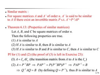
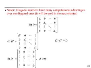
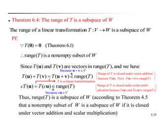
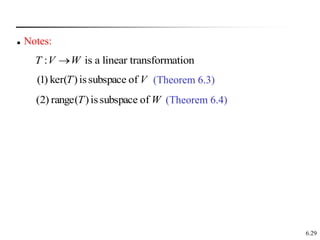
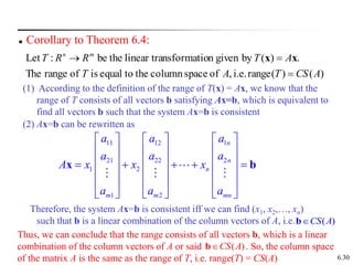
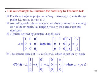
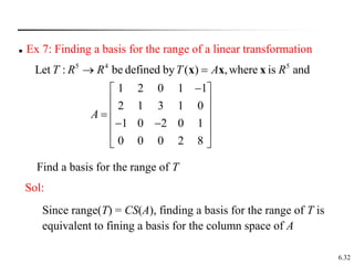
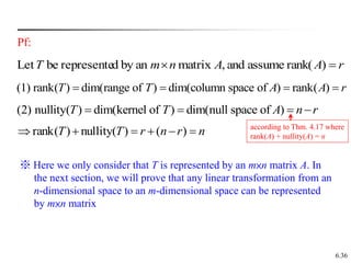
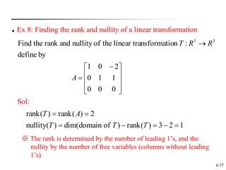
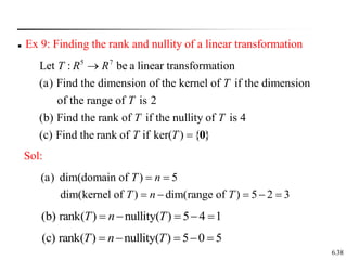
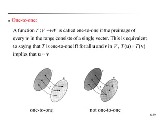
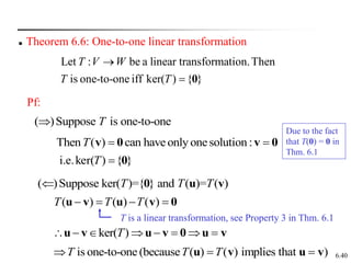
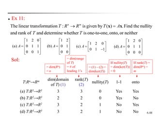
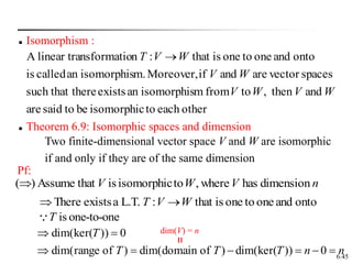
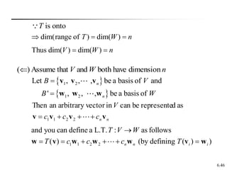
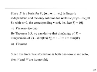
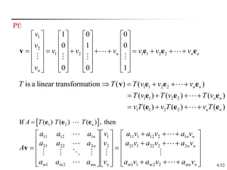
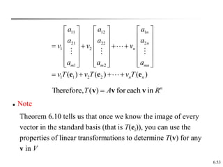
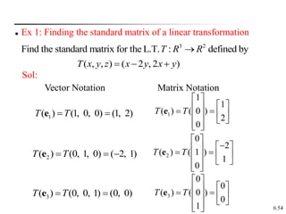
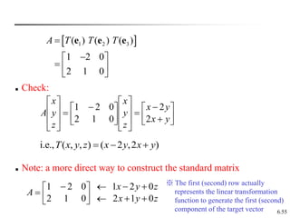
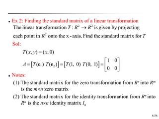
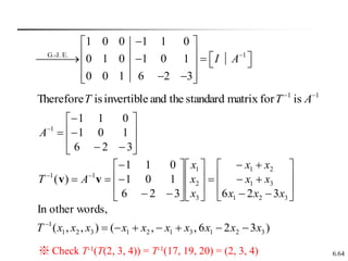
This document discusses linear transformations. It begins by defining a linear transformation as a function between vector spaces that preserves vector addition and scalar multiplication. It provides examples of linear transformations and functions that are not linear transformations. It then discusses properties of linear transformations including the zero and identity transformations. It introduces the concept that a linear transformation can be represented by a matrix and that matrix multiplication defines a linear transformation. It concludes by stating that a linear transformation defined by a matrix satisfies the properties of being linear.

1. Linear Transformations
6.1 Introduction to Linear Transformations
6.2 The Kernel and Range of a Linear Transformation
6.3 Matrices for Linear Transformations
6.4 Transition Matrices and Similarity
6.5 Applications of Linear Transformations
6.1

2. 6.2
6.1 Introduction to Linear Transformations
 A function T that maps a vector space V into a vector space W:
mapping
: , , : vector spaces
T V W V W

V: the domain of T W: the codomain of T
 Image of v under T :
If v is a vector in V and w is a vector in W such that
( ) ,
T 
v w
then w is called the image of v under T
(For each v, there is only one w)
 The range of T :
The set of all images of vectors in V (see the figure on the
next slide)

3. 6.3
※ For example, V is R3, W is R3, and T
is the orthogonal projection of any
vector (x, y, z) onto the xy-plane, i.e.
T(x, y, z) = (x, y, 0)
(we will use the above example many
times to explain abstract notions)
※ Then the domain is R3, the codomain
is R3, and the range is xy-plane (a
subspace of the codomian R3)
※ (2, 1, 0) is the image of (2, 1, 3)
※ The preimage of (2, 1, 0) is (2, 1, s),
where s is any real number
 The preimage of w:
The set of all v in V such that T(v)=w
(For each w, v may not be unique)
 The graphical representations of the domain, codomain, and range

4. 6.4
 Ex 1: A function from R2 into R2
2
2
: R
R
T 
)
2
,
(
)
,
( 2
1
2
1
2
1 v
v
v
v
v
v
T 


2
2
1 )
,
( R
v
v 

v
(a) Find the image of v=(-1,2) (b) Find the preimage of w=(-1,11)
Sol:
(a) ( 1, 2)
( ) ( 1, 2) ( 1 2, 1 2(2)) ( 3, 3)
T T
 
         
v
v
(b) ( ) ( 1, 11)
T   
v w
)
11
,
1
(
)
2
,
(
)
,
( 2
1
2
1
2
1 



 v
v
v
v
v
v
T
11
2
1
2
1
2
1






v
v
v
v
4
,
3 2
1 

 v
v Thus {(3, 4)} is the preimage of w=(-1, 11)

5. 6.5
 Linear Transformation :
true
are
properties
two
following
the
if
into
of
n
nsformatio
linear tra
A
：
:
spaces
vector
：
,
W
V
W
V
T
W
V

V
T
T
T 



 v
u
v
u
v
u ,
),
(
)
(
)
(
(1)
R
c
cT
c
T 

 ),
(
)
(
)
2
( u
u

6. 6.6
 Notes:
(1) A linear transformation is said to be operation preserving
)
(
)
(
)
( v
u
v
u T
T
T 


Addition
in V
Addition
in W
)
(
)
( u
u cT
c
T 
Scalar
multiplication
in V
Scalar
multiplication
in W
(2) A linear transformation from a vector space into
itself is called a linear operator
V
V
T 
:
(because the same result occurs whether the operations of addition
and scalar multiplication are performed before or after the linear
transformation is applied)

7. 6.7
 Ex 2: Verifying a linear transformation T from R2 into R2
Pf:
)
2
,
(
)
,
( 2
1
2
1
2
1 v
v
v
v
v
v
T 


number
real
any
:
,
in
vector
:
)
,
(
),
,
( 2
2
1
2
1 c
R
v
v
u
u 
 v
u
1 2 1 2 1 1 2 2
(1) Vector addition :
( , ) ( , ) ( , )
u u v v u v u v
     
u v
)
(
)
(
)
2
,
(
)
2
,
(
))
2
(
)
2
(
),
(
)
((
))
(
2
)
(
),
(
)
((
)
,
(
)
(
2
1
2
1
2
1
2
1
2
1
2
1
2
1
2
1
2
2
1
1
2
2
1
1
2
2
1
1
v
u
v
u
T
T
v
v
v
v
u
u
u
u
v
v
u
u
v
v
u
u
v
u
v
u
v
u
v
u
v
u
v
u
T
T



























8. 6.8
)
,
(
)
,
(
tion
multiplica
Scalar
)
2
(
2
1
2
1 cu
cu
u
u
c
c 

u
)
(
)
2
,
(
)
2
,
(
)
,
(
)
(
2
1
2
1
2
1
2
1
2
1
u
u
cT
u
u
u
u
c
cu
cu
cu
cu
cu
cu
T
c
T








Therefore, T is a linear transformation

9. 6.9
 Ex 3: Functions that are not linear transformations
(a) ( ) sin
f x x

2
(b) ( )
f x x

(c) ( ) 1
f x x
 
)
sin(
)
sin(
)
sin( 2
1
2
1 x
x
x
x 


)
sin(
)
sin(
)
sin( 3
2
3
2







2
2
2
1
2
2
1 )
( x
x
x
x 


2
2
2
2
1
)
2
1
( 


1
)
( 2
1
2
1 


 x
x
x
x
f
2
)
1
(
)
1
(
)
(
)
( 2
1
2
1
2
1 






 x
x
x
x
x
f
x
f
)
(
)
(
)
( 2
1
2
1 x
f
x
f
x
x
f 


(f(x) = sin x is not a linear transformation)
(f(x) = x2 is not a linear transformation)
(f(x) = x+1 is not a linear transformation,
although it is a linear function)
In fact, ( ) ( )
f cx cf x


10. 6.10
 Notes: Two uses of the term “linear”.
(1) is called a linear function because its graph
is a line
1
)
( 
 x
x
f
(2) is not a linear transformation from a vector
space R into R because it preserves neither vector
addition nor scalar multiplication
1
)
( 
 x
x
f

11. 6.11
 Zero transformation:
V
W
V
T 
 v
u,
,
:
( ) ,
T V
  
v 0 v
 Identity transformation:
V
V
T 
: V
T 

 v
v
v ,
)
(
 Theorem 6.1: Properties of linear transformations
W
V
T 
:
0
0 
)
(
(1)T
)
(
)
(
(2) v
v T
T 


)
(
)
(
)
(
(3) v
u
v
u T
T
T 


)
(
)
(
)
(
)
(
)
(
then
,
If
(4)
2
2
1
1
2
2
1
1
2
2
1
1
n
n
n
n
n
n
v
T
c
v
T
c
v
T
c
v
c
v
c
v
c
T
T
v
c
v
c
v
c















v
v
(T(cv) = cT(v) for c=-1)
(T(u+(-v))=T(u)+T(-v) and property (2))
(T(cv) = cT(v) for c=0)
(Iteratively using T(u+v)=T(u)+T(v) and T(cv) = cT(v))

12. 6.12
 Ex 4: Linear transformations and bases
Let be a linear transformation such that
3
3
: R
R
T 
)
4
,
1
,
2
(
)
0
,
0
,
1
( 

T
)
2
,
5
,
1
(
)
0
,
1
,
0
( 

T
)
1
,
3
,
0
(
)
1
,
0
,
0
( 
T
Sol:
)
1
,
0
,
0
(
2
)
0
,
1
,
0
(
3
)
0
,
0
,
1
(
2
)
2
,
3
,
2
( 



)
0
,
7
,
7
(
)
1
,
3
,
0
(
2
)
2
,
5
,
1
(
3
)
4
,
1
,
2
(
2
)
1
,
0
,
0
(
2
)
0
,
1
,
0
(
3
)
0
,
0
,
1
(
2
)
2
,
3
,
2
(










T
T
T
T
T
Find T(2, 3, -2)
1 1 2 2 1 1 2 2
According to the fourth property on the previous slide that
( ) ( ) ( ) ( )
n n n n
T c v c v c v c T v c T v c T v
 
 
      
 

13. 6.13
 Ex 5: A linear transformation defined by a matrix
The function is defined as
3
2
: R
R
T  

















2
1
2
1
1
2
0
3
)
(
v
v
A
T v
v
2 3
(a) Find ( ), where (2, 1)
(b) Show that is a linear transformation form into
T
T R R
 
v v
Sol:
(a) (2, 1)
 
v




























0
3
6
1
2
2
1
1
2
0
3
)
( v
v A
T
)
0
,
3
,
6
(
)
1
,
2
( 

T
vector
2
R vector
3
R
(b) ( ) ( ) ( ) ( )
T A A A T T
      
u v u v u v u v
)
(
)
(
)
(
)
( u
u
u
u cT
A
c
c
A
c
T 


(vector addition)
(scalar multiplication)

14. 6.14
 Theorem 6.2: The linear transformation defined by a matrix
Let A be an mn matrix. The function T defined by
v
v A
T 
)
(
is a linear transformation from Rn into Rm
 Note:















































n
mn
m
m
n
n
n
n
n
mn
m
m
n
n
v
a
v
a
v
a
v
a
v
a
v
a
v
a
v
a
v
a
v
v
v
a
a
a
a
a
a
a
a
a
A











2
2
1
1
2
2
22
1
21
1
2
12
1
11
2
1
2
1
2
22
21
1
12
11
v
v
v A
T 
)
( m
n
R
R
T 

:
vector
n
R vector
m
R
※ If T(v) can represented by Av, then T is a linear transformation
※ If the size of A is m×n, then the domain of T is Rn and the
codomain of T is Rm

15. 6.15
Show that the L.T. given by the matrix
has the property that it rotates every vector in R2
counterclockwise about the origin through the angle 
 Ex 7: Rotation in the plane
2
2
: R
R
T 





 





cos
sin
sin
cos
A
Sol:
( , ) ( cos , sin )
x y r r
 
 
v
(Polar coordinates: for every point on the xy-
plane, it can be represented by a set of (r, α))
r：the length of v ( )
：the angle from the positive
x-axis counterclockwise to
the vector v
2 2
x y
 
v
T(v)

16. 6.16





























 












 


)
sin(
)
cos(
sin
cos
cos
sin
sin
sin
cos
cos
sin
cos
cos
sin
sin
cos
cos
sin
sin
cos
)
(






















r
r
r
r
r
r
r
r
y
x
A
T v
v
r：remain the same, that means the length of T(v) equals the
length of v
 +：the angle from the positive x-axis counterclockwise to
the vector T(v)
Thus, T(v) is the vector that results from rotating the vector v
counterclockwise through the angle 
according to the addition
formula of trigonometric
identities

17. 6.17
is called a projection in R3
 Ex 8: A projection in R3
The linear transformation is given by
3
3
: R
R
T 









0
0
0
0
1
0
0
0
1
A
1 0 0
If is ( , , ), 0 1 0
0 0 0 0
x x
x y z A y y
z
     
     
 
     
     
     
v v
※ In other words, T maps every vector in R3
to its orthogonal projection in the xy-plane,
as shown in the right figure

18. 6.18
Keywords in Section 6.1:
 function
 domain
 codomain
 image of v under T
 range of T
 preimage of w
 linear transformation
 linear operator
 zero transformation
 identity transformation

19. 6.19
6.2 The Kernel and Range of a Linear Transformation
 Kernel of a linear transformation T :
Let be a linear transformation. Then the set of
all vectors v in V that satisfy is called the kernel
of T and is denoted by ker(T)
W
V
T 
:
0
v 
)
(
T
}
,
)
(
|
{
)
ker( V
T
T 


 v
0
v
v
※ For example, V is R3, W is R3, and T is the
orthogonal projection of any vector (x, y, z)
onto the xy-plane, i.e. T(x, y, z) = (x, y, 0)
※ Then the kernel of T is the set consisting of
(0, 0, s), where s is a real number, i.e.
ker( ) {(0,0, )| is a real number}
T s s


20. 6.20
 Ex 2: The kernel of the zero and identity transformations
(a) If T(v) = 0 (the zero transformation ), then
W
V
T 
:
V
T 
)
ker(
(b) If T(v) = v (the identity transformation ), then
V
V
T 
:
}
{
)
ker( 0

T

21. 6.21
 Ex 5: Finding the kernel of a linear transformation
1
3 2
2
3
1 1 2
( ) ( : )
1 2 3
x
T A x T R R
x
 
 
   
  
   

   
 
x x
?
)
ker( 
T
Sol:
3
1 2 3 1 2 3 1 2 3
ker( ) {( , , ) | ( , , ) (0,0), and ( , , ) }
T x x x T x x x x x x R
  
)
0
,
0
(
)
,
,
( 3
2
1 
x
x
x
T
























0
0
3
2
1
2
1
1
3
2
1
x
x
x

22. 6.22





























1
1
1
3
2
1
t
t
t
t
x
x
x
)}
1
,
1
,
1
span{(
}
number
real
a
is
|
)
1
,
1
,
1
(
{
)
ker(




 t
t
T
G.-J. E.
1 1 2 0 1 0 1 0
1 2 3 0 0 1 1 0
  
   


   

   

23. 6.23
 Theorem 6.3: The kernel is a subspace of V
The kernel of a linear transformation is a
subspace of the domain V
W
V
T 
:
)
1
6.
Theorem
by
(
)
( 0
0 
T

Pf:
V
T of
subset
nonempty
a
is
)
ker(

Then
.
of
kernel
in the
vectors
be
and
Let T
v
u
0
0
0
v
u
v
u 




 )
(
)
(
)
( T
T
T
0
0
u
u 

 c
cT
c
T )
(
)
(
Thus, ker( ) is a subspace of (according to Theorem 4.5
that a nonempty subset of is a subspace of if it is closed
under vector addition and scalar multiplication)
T V
V V
T is a linear transformation
( ker( ), ker( ) ker( ))
T T T
    
u v u v
( ker( ) ker( ))
T c T
  
u u

24. 6.24
 Ex 6: Finding a basis for the kernel


















8
2
0
0
0
1
0
2
0
1
0
1
3
1
2
1
1
0
2
1
and
in
is
where
,
)
(
by
defined
be
:
Let 5
4
5
A
R
A
T
R
R
T x
x
x
Find a basis for ker(T) as a subspace of R5
Sol:
To find ker(T) means to find all x satisfying T(x) = Ax = 0.
Thus we need to form the augmented matrix first
 
A 0

25. 6.25
 
G.-J. E.
1 2 0 1 1 0 1 0 2 0 1 0
2 1 3 1 0 0 0 1 1 0 2 0
1 0 2 0 1 0 0 0 0 1 4 0
0 0 0 2 8 0 0 0 0 0 0 0
A 
 
   
   
 
   


   
 
   
   
0
s t
1
2
3
4
5
2 2 1
2 1 2
1 0
4 0 4
0 1
x s t
x s t
x s t
s
x t
x t
  
       
       

       
       
   
       
 
       
       
     
 
x
  T
B of
kernel
for the
basis
one
:
)
1
,
4
,
0
,
2
,
1
(
),
0
,
0
,
1
,
1
,
2
( 



26. 6.26
 Corollary to Theorem 6.3:
0
x
x
x



A
T
A
T
R
R
T m
n
of
space
solution
the
to
equal
is
of
kernel
Then the
.
)
(
by
given
tion
fransforma
linear
the
be
:
Let
 
( ) (a linear transformation : )
ker( ) ( ) | 0, (subspace of )
n m
n n
T A T R R
T NS A A R R
 
     
x x
x x x
※ The kernel of T equals the nullspace of A (which is defined
in Theorem 4.16 on p.239) and these two are both subspaces
of Rn )
※ So, the kernel of T is sometimes called the nullspace of T

27. 6.27
 Range of a linear transformation T :
)
(
range
by
denoted
is
and
of
range
the
called
is
in
s
any vector
of
images
are
that
in
vectors
all
of
set
Then the
n.
nsformatio
linear tra
a
be
:
Let
T
T
V
W
W
V
T
w

}
|
)
(
{
)
(
range V
T
T 

 v
v
※ For the orthogonal projection of
any vector (x, y, z) onto the xy-
plane, i.e. T(x, y, z) = (x, y, 0)
※ The domain is V=R3, the codomain
is W=R3, and the range is xy-plane
(a subspace of the codomian R3)
※ Since T(0, 0, s) = (0, 0, 0) = 0, the
kernel of T is the set consisting of
(0, 0, s), where s is a real number

28. 6.28
W
W
V
T of
subspace
a
is
:
n
nsformatio
linear tra
a
of
range
The 
 Theorem 6.4: The range of T is a subspace of W
Pf:
( ) (Theorem 6.1)
T 
0 0
W
T of
subset
nonempty
a
is
)
(
range

have
we
and
),
range(
in
vectors
are
)
(
and
)
(
Since T
T
T v
u
)
(
range
)
(
)
(
)
( T
T
T
T 


 v
u
v
u
)
(
range
)
(
)
( T
c
T
cT 
 u
u
Thus, range( ) is a subspace of (according to Theorem 4.5
that a nonempty subset of is a subspace of if it is closed
under vector addition and scalar multiplication)
T W
W W
T is a linear transformation
Range of is closed under vector addition
because ( ), ( ), ( ) range( )
T
T T T T
 
 
 
 
u v u v
Range of is closed under scalar multi-
plication because ( ) and ( ) range( )
T
T T c T
 
 

 
u u
because V
 
u v
because c V

u

29. 6.29
 Notes:
of
subspace
is
)
ker(
)
1
( V
T
: is a linear transformation
T V W

of
subspace
is
)
(
range
)
2
( W
T
(Theorem 6.3)
(Theorem 6.4)

30. 6.30
 Corollary to Theorem 6.4:
)
(
)
(
range
i.e.
,
of
space
column
the
to
equal
is
of
range
The
.
)
(
by
given
n
nsformatio
linear tra
the
be
:
Let
A
CS
T
A
T
A
T
R
R
T m
n


 x
x
(1) According to the definition of the range of T(x) = Ax, we know that the
range of T consists of all vectors b satisfying Ax=b, which is equivalent to
find all vectors b such that the system Ax=b is consistent
(2) Ax=b can be rewritten as
Therefore, the system Ax=b is consistent iff we can find (x1, x2,…, xn)
such that b is a linear combination of the column vectors of A, i.e.
11 12 1
21 22 2
1 2
1 2
n
n
n
m m mn
a a a
a a a
A x x x
a a a
     
     
     
    
     
     
     
x b
Thus, we can conclude that the range consists of all vectors b, which is a linear
combination of the column vectors of A or said . So, the column space
of the matrix A is the same as the range of T, i.e. range(T) = CS(A)
( )
CS A

b
( )
CS A

b

31. 6.31
 Use our example to illustrate the corollary to Theorem 6.4:
※ For the orthogonal projection of any vector (x, y, z) onto the xy-
plane, i.e. T(x, y, z) = (x, y, 0)
※ According to the above analysis, we already knew that the range
of T is the xy-plane, i.e. range(T)={(x, y, 0)| x and y are real
numbers}
※ T can be defined by a matrix A as follows
※ The column space of A is as follows, which is just the xy-plane
1 0 0 1 0 0
0 1 0 , such that 0 1 0
0 0 0 0 0 0 0
x x
A y y
z
       
       
 
       
       
       
1
1 2 3 2 1 2
1 0 0
( ) 0 1 0 , where ,
0 0 0 0
x
CS A x x x x x x R
       
       
    
       
       
       

32. 6.32
 Ex 7: Finding a basis for the range of a linear transformation
5 4 5
Let : be defined by ( ) ,where is and
1 2 0 1 1
2 1 3 1 0
1 0 2 0 1
0 0 0 2 8
T R R T A R
A
 

 
 
 

 
 
 
 
x x x
Find a basis for the range of T
Sol:
Since range(T) = CS(A), finding a basis for the range of T is
equivalent to fining a basis for the column space of A

33. 6.33
G.-J. E.
1 2 0 1 1 1 0 2 0 1
2 1 3 1 0 0 1 1 0 2
1 0 2 0 1 0 0 0 1 4
0 0 0 2 8 0 0 0 0 0
A B
 
   
   

   
 
 
   
 
   
   
5
4
3
2
1 c
c
c
c
c 5
4
3
2
1 w
w
w
w
w
 
 
1 2 4 1 2 4
1 2 4 1 2 4
, , and are indepdnent, so , , can
form a basis for ( )
Row operations will not affect the dependency among columns
, , and are indepdnent, and thus , , is
a b
w w w w w w
CS B
c c c c c c


 
asis for ( )
That is, (1, 2, 1, 0), (2, 1, 0, 0), (1, 1, 0, 2) is a basis
for the range of
CS A
T


34. 6.34
 Rank of a linear transformation T:V→W :
rank( ) the dimension of the range of dim(range( ))
T T T
 
 Nullity of a linear transformation T:V→W :
nullity( ) the dimension of the kernel of dim(ker( ))
T T T
 
 Note:
If : is a linear transformation given by ( ) , then
dim(range( )) dim( ( ))
rank( ) rank( )
null dim(ker
ity( ) nullity
( )) dim( ( ) (
) )
n m
T R R T A
T CS A
T NS
T A
T A
A


 
 
 
x x
※ The dimension of the row (or column) space of a matrix A is called the rank of A
※ The dimension of the nullspace of A ( ) is called the nullity
of A
( ) { | 0}
NS A A
 
x x
According to the corollary to Thm. 6.3, ker(T) = NS(A), so dim(ker(T)) = dim(NS(A))
According to the corollary to Thm. 6.4, range(T) = CS(A), so dim(range(T)) = dim(CS(A))

35. 6.35
 Theorem 6.5: Sum of rank and nullity
(i.e. dim(range of ) dim(kernel of
rank( )
)
n
dim(domain o
ullity
f ))
)
(
T
T
T T
T n
 
 
Let T: V →W be a linear transformation from an n-dimensional
vector space V (i.e. the dim(domain of T) is n) into a vector
space W. Then
※ You can image that the dim(domain of T)
should equals the dim(range of T)
originally
※ But some dimensions of the domain of T
is absorbed by the zero vector in W
※ So the dim(range of T) is smaller than
the dim(domain of T) by the number of
how many dimensions of the domain of
T are absorbed by the zero vector,
which is exactly the dim(kernel of T)

36. 6.36
Pf:
r
A
A
n
m
T 
 )
rank(
assume
and
,
matrix
an
by
d
represente
be
Let
(1) rank( ) dim(range of ) dim(column space of ) rank( )
T T A A r
   
n
r
n
r
T
T 




 )
(
)
(
nullity
)
(
rank
(2) nullity( ) dim(kernel of ) dim(null space of )
T T A n r
   
※ Here we only consider that T is represented by an m×n matrix A. In
the next section, we will prove that any linear transformation from an
n-dimensional space to an m-dimensional space can be represented
by m×n matrix
according to Thm. 4.17 where
rank(A) + nullity(A) = n

37. 6.37
 Ex 8: Finding the rank and nullity of a linear transformation









 


0
0
0
1
1
0
2
0
1
by
define
:
n
nsformatio
linear tra
the
of
nullity
and
rank
the
Find 3
3
A
R
R
T
Sol:
1
2
3
)
(
rank
)
of
domain
dim(
)
(
nullity
2
)
(
rank
)
(
rank







T
T
T
A
T
※ The rank is determined by the number of leading 1’s, and the
nullity by the number of free variables (columns without leading
1’s)

38. 6.38
 Ex 9: Finding the rank and nullity of a linear transformation
5 7
Let : be a linear transformation
(a) Find the dimension of the kernel of if the dimension
of the range of is 2
(b) Find the rank of if the nullity of is 4
(c) Find the rank of if ke
T R R
T
T
T T
T

r( ) { }
T  0
Sol:
(a) dim(domain of ) 5
dim(kernel of ) dim(range of ) 5 2 3
T n
T n T
 
    
(b) rank( ) nullity( ) 5 4 1
T n T
    
(c) rank( ) nullity( ) 5 0 5
T n T
    

39. 6.39
A function : is called one-to-one if the preimage of
every in the range consists of a single vector. This is equivalent
to saying that is one-to-one iff for all and in , ( ) ( )
implies
T V W
T V T T


w
u v u v
that 
u v
 One-to-one:
one-to-one not one-to-one

40. 6.40
 Theorem 6.6: One-to-one linear transformation
Let : be a linear transformation.Then
is one-to-one iff ker( ) { }
T V W
T T

 0
Pf:
( )Suppose is one-to-one
T

Then ( ) can haveonly onesolution :
T  
v 0 v 0
}
{
)
ker(
i.e. 0

T
( )Suppose ker( )={ } and ( )= ( )
T T T
 0 u v
0
v
u
v
u 


 )
(
)
(
)
( T
T
T
ker( )
T
       
u v u v 0 u v
is one-to-one (because ( ) ( ) implies that )
T T T
  
u v u v
T is a linear transformation, see Property 3 in Thm. 6.1
Due to the fact
that T(0) = 0 in
Thm. 6.1

41. 6.41
 Ex 10: One-to-one and not one-to-one linear transformation
(a) The linear transformation : given by ( )
is one-to-one
T
m n n m
T M M T A A
 
 
3 3
(b) The zero transformation : is not one-to-one
T R R

because its kernel consists of only the m×n zero matrix
because its kernel is all of R3

42. 6.42
in
preimage
a
has
in
element
every
if
onto
be
to
said
is
:
function
A
V
W
W
V
T 
 Onto:
(T is onto W when W is equal to the range of T)
 Theorem 6.7: Onto linear transformations
Let T: V → W be a linear transformation, where W is finite
dimensional. Then T is onto if and only if the rank of T is equal
to the dimension of W
)
dim(
)
of
range
dim(
)
(
rank W
T
T 

The definition of
the rank of a linear
transformation
The definition
of onto linear
transformations

43. 6.43
 Theorem 6.8: One-to-one and onto linear transformations
Let : be a linear transformation with vector space and
both of dimension .Then is one-to-one if and only if it is onto
T V W V W
n T

Pf:
( ) If is one-to-one, then ker( ) { }and dim(ker( )) 0
T T T
  
0
)
dim(
))
dim(ker(
))
(
range
dim(
6.5
Thm.
W
n
T
n
T 



Consequently, is onto
T
}
{
)
ker(
0
)
of
range
dim(
))
dim(ker(
6.5
Thm.
0






 T
n
n
T
n
T
Therefore, is one-to-one
T
n
W
T
T 

 )
dim(
)
of
range
dim(
then
onto,
is
If
)
(
According to the definition of dimension
(on p.227) that if a vector space V
consists of the zero vector alone, the
dimension of V is defined as zero

44. 6.44
 Ex 11:
The linear transformation : is given by ( ) .Find the nullity
and rank of and determine whether is one-to-one, onto, or neither
n m
T R R T A
T T
 
x x
1 2 0
(a) 0 1 1
0 0 1
A
 
 
  
 
 
1 2
(b) 0 1
0 0
A
 
 
  
 
 
1 2 0
(c)
0 1 1
A
 
  

 
1 2 0
(d) 0 1 1
0 0 0
A
 
 
  
 
 
Sol:
T:Rn→Rm dim(domain
of T) (1)
rank(T)
(2)
nullity(T) 1-1 onto
(a) T:R3→R3 3 3 0 Yes Yes
(b) T:R2→R3 2 2 0 Yes No
(c) T:R3→R2 3 2 1 No Yes
(d) T:R3→R3 3 2 1 No No
= dim(range
of T)
= # of
leading 1’s
= (1) – (2) =
dim(ker(T))
If nullity(T)
= dim(ker(T))
= 0
If rank(T) =
dim(Rm) =
m
= dim(Rn)
= n

45. 6.45
 Isomorphism :
other
each
to
isomorphic
be
to
said
are
and
then
,
to
from
m
isomorphis
an
exists
there
such that
spaces
vector
are
and
if
Moreover,
m.
isomorphis
an
called
is
onto
and
one
to
one
is
that
:
n
nsformatio
linear tra
A
W
V
W
V
W
V
W
V
T 
 Theorem 6.9: Isomorphic spaces and dimension
Pf:
n
V
W
V dimension
has
where
,
to
isomorphic
is
that
Assume
)
(
onto
and
one
to
one
is
that
:
L.T.
a
exists
There W
V
T 

is one-to-one
T
n
n
T
T
T
T








0
))
dim(ker(
)
of
domain
dim(
)
of
range
dim(
0
))
dim(ker(
Two finite-dimensional vector space V and W are isomorphic
if and only if they are of the same dimension
dim(V) = n

46. 6.46
n
W
V dimension
have
both
and
that
Assume
)
(
is onto
T
n
W
T 

 )
dim(
)
of
range
dim(
n
W
V 
 )
dim(
)
dim(
Thus
 
 
1 2
1 2
Let , , , be a basis of and
' , , , be a basis of
n
n
B V
B W


v v v
w w w
n
n
c
c
c
V
v
v
v
v 


 
2
2
1
1
as
d
represente
be
can
in
vector
arbitrary
an
Then
1 1 2 2
and you can define a L.T. : as follows
( ) (by defining ( ) )
n n i i
T V W
T c c c T

     
w v w w w v w

47. 6.47
Since is a basis for V, {w1, w2,…wn} is linearly
independent, and the only solution for w=0 is c1=c2=…=cn=0
So with w=0, the corresponding v is 0, i.e., ker(T) = {0}
By Theorem 6.5, we can derive that dim(range of T) =
dim(domain of T) – dim(ker(T)) = n –0 = n = dim(W)
Since this linear transformation is both one-to-one and onto,
then V and W are isomorphic
'
B
one
-
to
-
one
is
T

onto
is
T


48. 6.48
 Ex 12: (Isomorphic vector spaces)
4
(a) 4-space
R 
4 1
(b) space of all 4 1 matrices
M   
2 2
(c) space of all 2 2 matrices
M   
3
(d) ( ) space of all polynomials of degree 3 or less
P x 
5
1 2 3 4
(e) {( , , , , 0), are real numbers}(a subspace of )
i
V x x x x x R

The following vector spaces are isomorphic to each other
 Note
Theorem 6.9 tells us that every vector space with dimension
n is isomorphic to Rn

49. 6.49
Keywords in Section 6.2:
 kernel of a linear transformation T
 range of a linear transformation T
 rank of a linear transformation T
 nullity of a linear transformation T
 one-to-one
 onto
 Isomorphism (one-to-one and onto)
 isomorphic space

50. 6.50
6.3 Matrices for Linear Transformations
1 2 3 1 2 3 1 2 3 2 3
(1) ( , , ) (2 , 3 2 ,3 4 )
T x x x x x x x x x x x
      
 Three reasons for matrix representation of a linear transformation:
1
2
3
2 1 1
(2) ( ) 1 3 2
0 3 4
x
T A x
x

   
   
   
   
   
   
x x
 It is simpler to write
 It is simpler to read
 It is more easily adapted for computer use
 Two representations of the linear transformation T:R3→R3 :

51. 6.51
 Theorem 6.10: Standard matrix for a linear transformation
Let : be a linear trtansformation such that
n m
T R R

11 12 1
21 22 2
1 2
1 2
( ) , ( ) , , ( ) ,
n
n
n
m m mn
a a a
a a a
T T T
a a a
     
     
     
  
     
     
     
e e e
1 2 n
where{ , , , }is a standard basis for .Then the
matrix whose columns correspond to ( ),
n
i
R m n
n T

e e e
e
 
11 12 1
21 22 2
1 2
1 2
( ) ( ) ( ) ,
n
n
n
m m mn
a a a
a a a
A T T T
a a a
 
 
 
 
 
 
 
e e e
is such that 𝑇 𝐯 = 𝐴𝐯 for every 𝐯 in 𝑅𝑛, 𝐴 is called the
Standard matrix for T

52. 6.52
Pf:
1
2
1 2 1 1 2 2
1 0 0
0 1 0
0 0 1
n n n
n
v
v
v v v v v v
v
       
       
       
        
       
       
     
 
v e e e
1 1 2 2
1 1 2 2
1 1
is a linear transformation ( ) ( )
( ) ( ) ( )
( )
n n
n n
T T T v v v
T v T v T v
v T
    
   
 
v e e e
e e e
e 2 2
( ) ( )
n n
v T v T
 
e e















































n
mn
m
m
n
n
n
n
n
mn
m
m
n
n
v
a
v
a
v
a
v
a
v
a
v
a
v
a
v
a
v
a
v
v
v
a
a
a
a
a
a
a
a
a
A












2
2
1
1
2
2
22
1
21
1
2
12
1
11
2
1
2
1
2
22
21
1
12
11
v
 
1 2
If ( ) ( ) ( ) , then
n
A T T T
 e e e

53. 6.53
11 12 1
21 22 2
1 2
1 2
1 1 2 2
( ) ( ) ( )
n
n
n
m m mn
n n
a a a
a a a
v v v
a a a
v T v T v T
     
     
     
   
     
     
     
   
e e e
n
R
A
T in
each
for
)
(
Therefore, v
v
v 
 Note
Theorem 6.10 tells us that once we know the image of every
vector in the standard basis (that is T(ei)), you can use the
properties of linear transformations to determine T(v) for any
v in V

54. 6.54
 Ex 1: Finding the standard matrix of a linear transformation
3 2
Find the standard matrix for the L.T. : defined by
T R R

)
2
,
2
(
)
,
,
( y
x
y
x
z
y
x
T 


Sol:
1
( ) (1, 0, 0) (1, 2)
T T
 
e
2
( ) (0, 1, 0) ( 2, 1)
T T
  
e
3
( ) (0, 0, 1) (0, 0)
T T
 
e
1
1
1
( ) ( 0 )
2
0
T T
 
 
 
   
 
 
 
 
e
2
0
2
( ) ( 1 )
1
0
T T
 

 
 
   
 
 
 
 
e
3
0
0
( ) ( 0 )
0
1
T T
 
 
 
   
 
 
 
 
e
Vector Notation Matrix Notation

55. 6.55
 
1 2 3
( ) ( ) ( )
1 2 0
2 1 0
A T T T


 
  
 
e e e
 Note: a more direct way to construct the standard matrix
z
y
x
z
y
x
A
0
1
2
0
2
1
0
1
2
0
2
1











 























 









y
x
y
x
z
y
x
z
y
x
A
2
2
0
1
2
0
2
1
i.e., ( , , ) ( 2 ,2 )
T x y z x y x y
  
 Check:
※ The first (second) row actually
represents the linear transformation
function to generate the first (second)
component of the target vector

56. 6.56
 Ex 2: Finding the standard matrix of a linear transformation
2 2
2
The linear transformation : is given by projecting
each point in onto the x -axis.Find the standard matrix for
T R R
R T

Sol:
)
0
,
(
)
,
( x
y
x
T 
   
1 2
1 0
( ) ( ) (1, 0) (0, 1)
0 0
A T T T T
 
    
 
e e
 Notes:
(1) The standard matrix for the zero transformation from Rn into Rm
is the mn zero matrix
(2) The standard matrix for the identity transformation from Rn into
Rn is the nn identity matrix In

57. 6.57
 Composition of T1:Rn→Rm with T2:Rm→Rp :
n
R
T
T
T 
 v
v
v )),
(
(
)
( 1
2
2 1
This composition is denoted by T T T

 Theorem 6.11: Composition of linear transformations
1 2
1 2
Let : and : be linear transformations
with standard matrices and ,then
n m m p
T R R T R R
A A
 
2 1
(1) The composition : , defined by ( ) ( ( )),
is still a linear transformation
n p
T R R T T T
 
v v
2 1
(2) The standard matrix for is given by the matrix product
A T
A A A


58. 6.58
Pf:
(1) ( is a linear transformation)
Let and be vectors in and let be any scalar.Then
n
T
R c
u v
2 1
(2) ( is thestandard matrix for )
A A T
)
(
)
(
))
(
(
))
(
(
))
(
)
(
(
))
(
(
)
(
1
2
1
2
1
1
2
1
2
v
u
v
u
v
u
v
u
v
u
T
T
T
T
T
T
T
T
T
T
T
T









)
(
))
(
(
))
(
(
))
(
(
)
( 1
2
1
2
1
2 v
v
v
v
v cT
T
cT
cT
T
c
T
T
c
T 



v
v
v
v
v )
(
)
(
))
(
(
)
( 1
2
1
2
1
2
1
2 A
A
A
A
A
T
T
T
T 



 Note:
1
2
2
1 T
T
T
T 
 

59. 6.59
 Ex 3: The standard matrix of a composition
3 3
1 2
Let and be linear transformations from into s.t.
T T R R
)
,
0
,
2
(
)
,
,
(
1 z
x
y
x
z
y
x
T 


)
,
z
,
(
)
,
,
(
2 y
y
x
z
y
x
T 

2 1
1 2
Find the standard matrices for the compositions
and '
T T T
T T T


Sol:
)
for
matrix
standard
(
1
0
1
0
0
0
0
1
2
1
1 T
A











)
for
matrix
standard
(
0
1
0
1
0
0
0
1
1
2
2 T
A









 


60. 6.60
1
2
for
matrix
standard
The T
T
T 

2
1
'
for
matrix
standard
The T
T
T 

























 


0
0
0
1
0
1
0
1
2
1
0
1
0
0
0
0
1
2
0
1
0
1
0
0
0
1
1
1
2 A
A
A









 










 












0
0
1
0
0
0
1
2
2
0
1
0
1
0
0
0
1
1
1
0
1
0
0
0
0
1
2
' 2
1A
A
A

61. 6.61
 Inverse linear transformation:
1 2
If : and : are L.T.s.t.for every in
n n n n n
T R R T R R R
  v
))
(
(
and
))
(
( 2
1
1
2 v
v
v
v 
 T
T
T
T
invertible
be
to
said
is
and
of
inverse
the
called
is
Then 1
1
2 T
T
T
 Note:
If the transformation T is invertible, then the inverse is
unique and denoted by T–1

62. 6.62
 Theorem 6.12: Existence of an inverse transformation
Let : be a linear transformation with standard matrix ,
Then the following condition are equivalent
n n
T R R A

 Note:
If T is invertible with standard matrix A, then the standard
matrix for T–1 is A–1
(1) T is invertible
(2) T is an isomorphism
(3) A is invertible
※ For (2)  (1), you can imagine that
since T is one-to-one and onto, for every
w in the codomain of T, there is only one
preimage v, which implies that T-1(w) =v
can be a L.T. and well-defined, so we can
infer that T is invertible
※ On the contrary, if there are many
preimages for each w, it is impossible to
find a L.T to represent T-1 (because for a
L.T, there is always one input and one
output), so T cannot be invertible

63. 6.63
 Ex 4: Finding the inverse of a linear transformation
3 3
Thelinear transformation : is defined by
T R R

)
4
2
,
3
3
,
3
2
(
)
,
,
( 3
2
1
3
2
1
3
2
1
3
2
1 x
x
x
x
x
x
x
x
x
x
x
x
T 






Sol:
1
4
2
1
3
3
1
3
2
for
matrix
standard
The











A
T
3
2
1
3
2
1
3
2
1
4
2
3
3
3
2
x
x
x
x
x
x
x
x
x









 









1
0
0
1
4
2
0
1
0
1
3
3
0
0
1
1
3
2
3
I
A
Show that T is invertible, and find its inverse

64. 6.64
G.-J. E. 1
1 0 0 1 1 0
0 1 0 1 0 1
0 0 1 6 2 3
I A

 
   

    
 
 
 
 
1
1
is
for
matrix
standard
the
and
invertible
is
Therefore 

A
T
T














3
2
6
1
0
1
0
1
1
1
A




































 

3
2
1
3
1
2
1
3
2
1
1
1
3
2
6
3
2
6
1
0
1
0
1
1
)
(
x
x
x
x
x
x
x
x
x
x
A
T v
v
)
3
2
6
,
,
(
)
,
,
(
s,
other word
In
3
2
1
3
1
2
1
3
2
1
1
x
x
x
x
x
x
x
x
x
x
T 







※ Check T-1(T(2, 3, 4)) = T-1(17, 19, 20) = (2, 3, 4)

65. 6.65
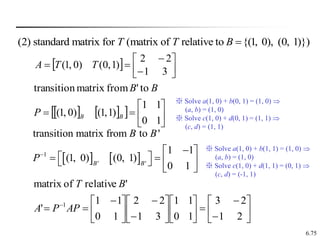
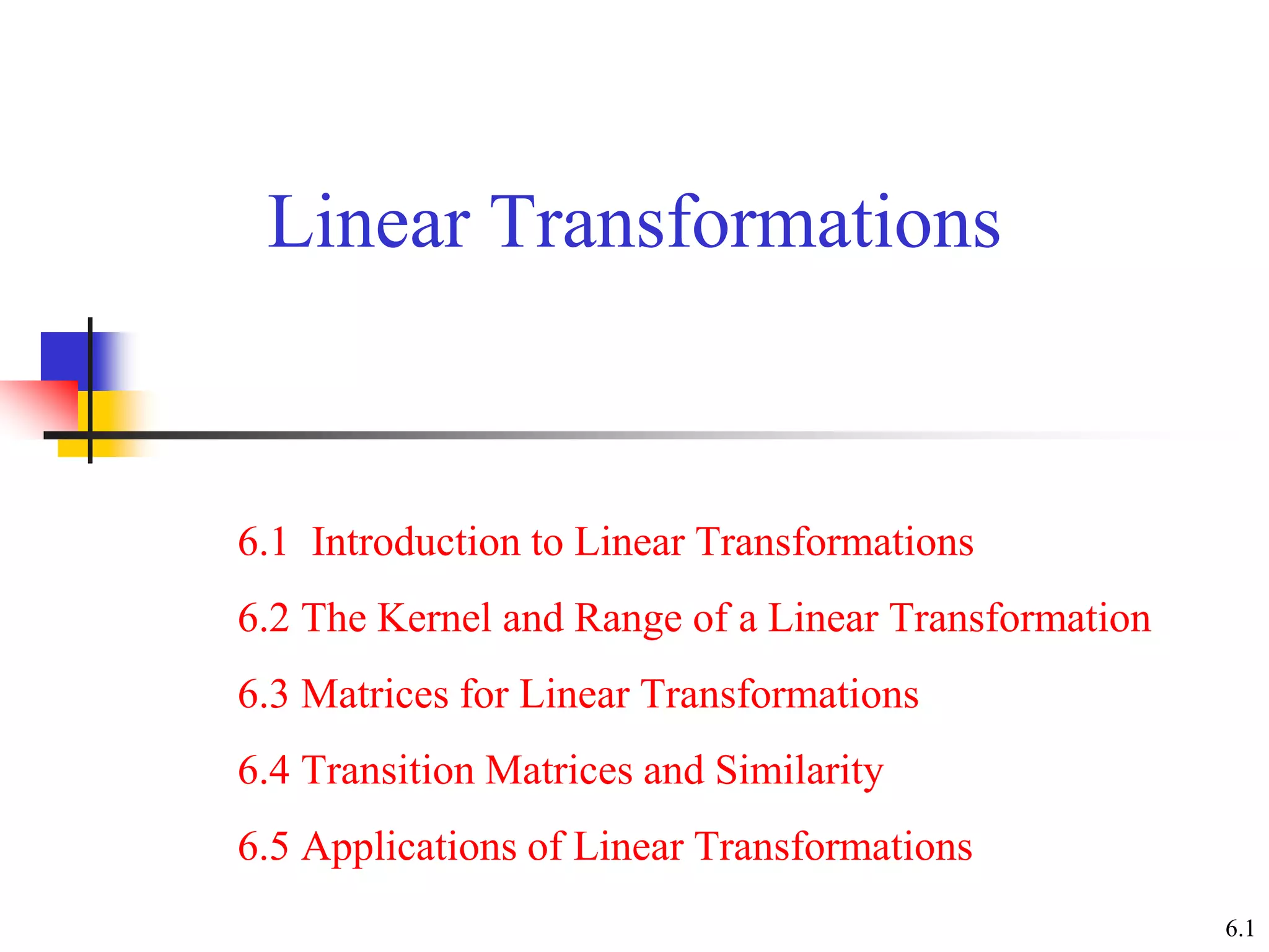
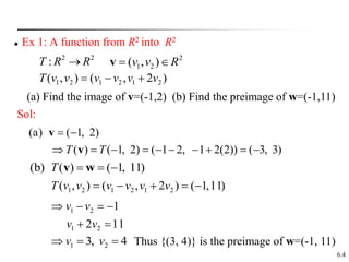
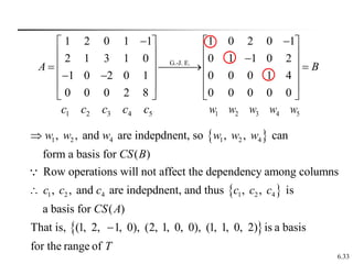
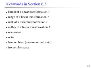
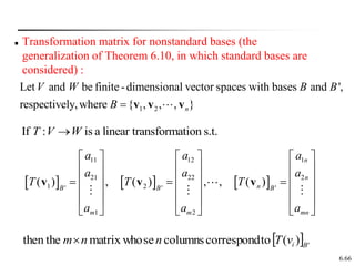
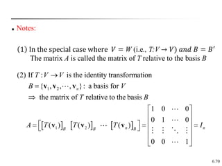
 The matrix of T relative to the bases B and B‘:
1 2
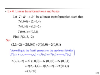
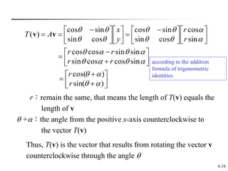
: (a linear transformation)
{ , , , } (a nonstandard basis for )
The coordinate matrix of any relative to is denoted by [ ]
n
B
T V W
B V
B

 v v v
v v
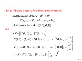
A matrix A can represent T if the result of A multiplied by a
coordinate matrix of v relative to B is a coordinate matrix of v
relative to B’, where B’ is a basis for W. That is,
where A is called the matrix of T relative to the bases B and B’
  '
( ) [ ] ,
B
B
T A

v v
1
2
1 1 2 2
if can be represeted as , then [ ]
n n B
n
c
c
c c c
c
 
 
 
 
 
 
   
 
 
 
 
 
 
 
v v v v v

66. 6.66
 Transformation matrix for nonstandard bases (the
generalization of Theorem 6.10, in which standard bases are
considered) :
     
11 12 1
21 22 2
1 2
' ' '
1 2
( ) , ( ) , , ( )
n
n
n
B B B
m m mn
a a a
a a a
T T T
a a a
     
     
     
  
     
     
     
v v v
1 2
Let and be finite-dimensional vector spaces with bases and ',
respectively,where { , , , }
n
V W B B
B  v v v
If : is a linear transformation s.t.
T V W

  '
)
(
to
correspond
columns
se
matrix who
then the B
i
v
T
n
n
m

67. 6.67
  '
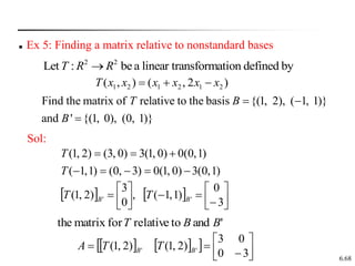
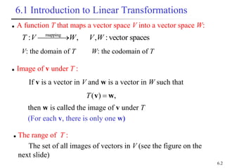
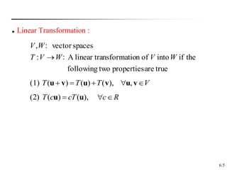
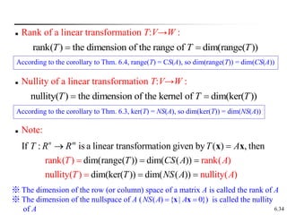
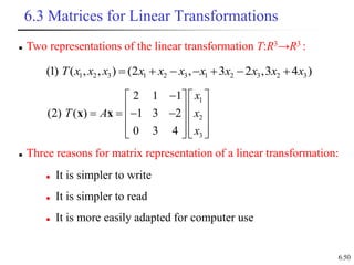
is such that ( ) [ ] for every in
B
B
T A V

v v v
 
11 12 1
21 22 2
1 2
1 2
[ ( )] [ ( )] [ ( )]
n
n
B B n B
m m mn
a a a
a a a
A T T T
a a a
  
 
 
 
 
 
 
 
v v v
※The above result state that the coordinate of T(v) relative to the basis B’
equals the multiplication of A defined above and the coordinate of v
relative to the basis B.
※ Comparing to the result in Thm. 6.10 (T(v) = Av), it can infer that the
linear transformation and the basis change can be achieved in one step
through multiplying the matrix A defined above (see the figure on 6.74
for illustration)

68. 6.68
 Ex 5: Finding a matrix relative to nonstandard bases
2 2
Let : bea linear transformation defined by
T R R

)
2
,
(
)
,
( 2
1
2
1
2
1 x
x
x
x
x
x
T 


Find the matrix of relative to the basis {(1, 2), ( 1, 1)}
and ' {(1, 0), (0, 1)}
T B
B
 

Sol:
)
1
,
0
(
3
)
0
,
1
(
0
)
3
,
0
(
)
1
,
1
(
)
1
,
0
(
0
)
0
,
1
(
3
)
0
,
3
(
)
2
,
1
(








T
T
    















3
0
)
1
,
1
(
,
0
3
)
2
,
1
( '
' B
B T
T
'
and
to
relative
for
matrix
the B
B
T
   
  








3
0
0
3
)
2
,
1
(
)
2
,
1
( '
' B
B T
T
A

69. 6.69
 Ex 6:
2 2
For the L.T. : given in Example 5, use the matrix
to find ( ),where (2, 1)
T R R A
T


v v
Sol:
)
1
,
1
(
1
)
2
,
1
(
1
)
1
,
2
( 



v
  








1
1
B
v
    























3
3
1
1
3
0
0
3
)
( ' B
B A
T v
v
)
3
,
3
(
)
1
,
0
(
3
)
0
,
1
(
3
)
( 


 v
T )}
1
,
0
(
),
0
,
1
{(
'
B
)}
1
,
1
(
),
2
,
1
{( 

B
)
3
,
3
(
)
1
2(2)
,
1
2
(
)
1
,
2
( 



T
 Check:

70. 6.70
 Notes:
     
1 2
1 2
(2) If : is the identity transformation
{ , , , }: a basis for
the matrix of relative to the basis
1 0 0
0 1 0
( ) ( ) ( )
0 0 1
n
n n
B B B
T V V
B V
T B
A T T T I



 
 
 
 
  
   
 
 
v v v
v v v
1 In the special case where 𝑉 = W (i.e., T:V → 𝑉) 𝑎𝑛𝑑 𝐵 = 𝐵′
The matrix A is called the matrix of T relative to the basis B

71. 6.71
Keywords in Section 6.3:
 standard matrix for T
 composition of linear transformations
 inverse linear transformation
 matrix of T relative to the bases B and B'
 matrix of T relative to the basis B:

72. 6.72
6.4 Transition Matrices and Similarity
1 2
1 2
: ( a linear transformation)
{ , , , } ( a basis of )
' { , , , } (a basis of )
n
n
T V V
B V
B V



v v v
w w w
     
1 2
( ) ( ) ( ) ( matrix of relative to )
n
B B B
A T T T T B
 
  
v v v
     
1 2
' ' '
' ( ) ( ) ( ) (matrix of relative to ')
n
B B B
A T T T T B
 
  
w w w
     
1 2 ( transition matrix from ' to )
n
B B B
P B B
 
  
w w w
     
1
1 2
' ' '
( transition matrix from to ')
n
B B B
P B B

 
  
v v v
from the definition of the transition matrix on p.254 in the
text book or on Slide 4.108 and 4.109 in the lecture notes
       
1
' '
, and
B B B B
P P
  
v v v v
       
' '
( ) , and ( )
B B B B
T A T A
  
v v v v

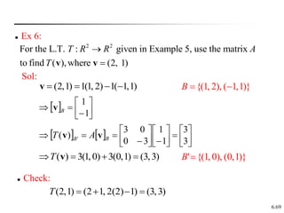
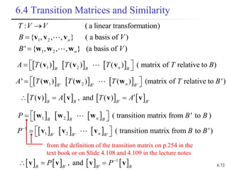
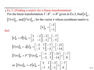
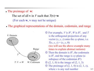
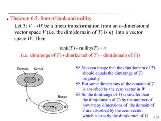
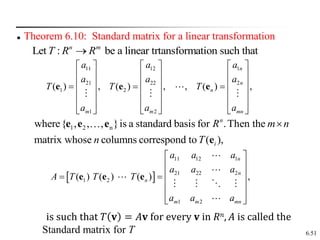
73. 6.73
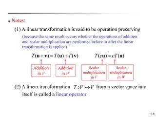
 Two ways to get from to :
' '
(1) (direct): '[ ] [ ( )]
B B
A T

v v
  '
B
v   '
)
( B
T v
1 1
' '
(2) (indirect): [ ] [ ( )] '
B B
P AP T A P AP
 
  
v v
direct
indirect

74. 6.74
 Ex 1: (Finding a matrix for a linear transformation)
Sol:
  












1
3
)
0
,
1
(
)
1
,
1
(
1
)
0
,
1
(
3
)
1
,
2
(
)
0
,
1
( '
B
T
T
2
2
：
for
matrix
the
Find R
R
T
A' 
)
3
,
2
2
(
)
,
( 2
1
2
1
2
1 x
x
x
x
x
x
T 



)}
1
,
1
(
),
0
,
1
{(
'
basis
the
to
reletive 
B
  











2
2
)
1
,
1
(
)
1
,
1
(
2
)
0
,
1
(
2
)
2
,
0
(
)
1
,
1
( '
B
T
T
   
  










2
1
2
3
)
1
,
1
(
)
0
,
1
(
' '
' B
B T
T
A
   
' '
(1) ' (1, 0) (1, 1)
B B
A T T
 
  

75. 6.75
(2) standard matrix for (matrix of relative to {(1, 0), (0, 1)})
T T B 
  









3
1
2
2
)
1
,
0
(
)
0
,
1
( T
T
A
   
  







1
0
1
1
)
1
,
1
(
)
0
,
1
(
to
'
from
matrix
transition
B
B
P
B
B
   
1
' '
transition matrix from to '
1 1
(1, 0) (0, 1)
0 1
B B
B B
P 
 
 
   
 
 




























 

 
2
1
2
3
1
0
1
1
3
1
2
2
1
0
1
1
'
'
relative
of
matrix
1
AP
P
A
B
T
※ Solve a(1, 0) + b(1, 1) = (1, 0) 
(a, b) = (1, 0)
※ Solve c(1, 0) + d(1, 1) = (0, 1) 
(c, d) = (-1, 1)
※ Solve a(1, 0) + b(0, 1) = (1, 0) 
(a, b) = (1, 0)
※ Solve c(1, 0) + d(0, 1) = (1, 1) 
(c, d) = (1, 1)

76. 6.76
 Ex 2: (Finding a matrix for a linear transformation)
Sol:
2 2 2
Let {( 3, 2), (4, 2)} and ' {( 1, 2), (2, 2)}be basis for
2 7
, and let be the matrix for : relative to .
3 7
Find the matrix of relative to '
B B
R A T R R B
T B
     

 
 
 

 
   
  











1
2
2
3
)
2
,
2
(
)
2
,
1
(
:
to
'
from
matrix
transition B
B
P
B
B
   
  












3
2
2
1
)
2
,
4
(
)
2
,
3
(
:
'
to
from
matrix
transition '
'
1
B
B
P
B
B

































 
3
1
1
2
1
2
2
3
7
3
7
2
3
2
2
1
'
:
'
to
relative
of
matrix
1
AP
P
A
B
T
Because the specific function is unknown, it is difficult to apply
the direct method to derive A’, so we resort to the indirect
method where A’ = P-1AP

77. 6.77
 Ex 3: (Finding a matrix for a linear transformation)
Sol:
 
   
 
2 2
'
'
For the linear transformation : given in Ex.2, find ,
( ) , and ( ) , for the vector whose coordinate matrix is
3
1
B
B B
B
T R R
T T


 
  

 
v
v v v
v
    


























5
7
1
3
1
2
2
3
'
B
B P v
v
    


























14
21
5
7
7
3
7
2
)
( B
B A
T v
v
    























 
0
7
14
21
3
2
2
1
)
(
)
( 1
' B
B T
P
T v
v
    























0
7
1
3
3
1
1
2
'
)
(
or '
' B
B A
T v
v

78. 6.78
 Similar matrix :
 For square matrices A and A’ of order n, A’ is said to be similar
to A if there exist an invertible matrix P s.t. A’=P-1AP
 Theorem 6.13: (Properties of similar matrices)
Let A, B, and C be square matrices of order n.
Then the following properties are true.
(1) A is similar to A
(2) If A is similar to B, then B is similar to A
(3) If A is similar to B and B is similar to C, then A is similar to C
Pf for (1) and (2) (the proof of (3) is left in Exercise 23):
(1) (the transition matrix from to is the )
n n n
A I AI A A I

1 1 1 1 1
1 1
(2) ( )
(by defining ), thus is similar to
A P BP PAP P P BP P PAP B
Q AQ B Q P B A
    
 
    
  

79. 6.79
 Ex 4: (Similar matrices)
2 2 3 2
(a) and ' are similar
1 3 1 2
A A
 
   
 
   
 
   







 
1
0
1
1
where
,
'
because 1
P
AP
P
A
2 7 2 1
(b) and ' are similar
3 7 1 3
A A

   
 
   
 
   









 
1
2
2
3
where
,
'
because 1
P
AP
P
A

80. 6.80
 Ex 5: (A comparison of two matrices for a linear transformation)
3 3
1 3 0
Suppose 3 1 0 is the matrix for : relative
0 0 2
to the standard basis.Find the matrix for relative to the basis
' {(1, 1, 0), (1, 1, 0), (0, 0, 1)}
A T R R
T
B
 
 
 
 
 

 
 
Sol:
     
 














1
0
0
0
1
1
0
1
1
)
1
,
0
,
0
(
)
0
,
1
,
1
(
)
0
,
1
,
1
(
matrix
standard
the
to
from
matrix
n
transitio
The
B
B
B
P
B'










 
1
0
0
0
0
2
1
2
1
2
1
2
1
1
P

81. 6.81
1 1
2 2
1 1 1
2 2
matrix of relative to ':
0 1 3 0 1 1 0
' 0 3 1 0 1 1 0
0 0 1 0 0 2 0 0 1
4 0 0
0 2 0
0 0 2
T B
A P AP

     
     
   
     
     

   
 
 
 
 
 
 

 
※ You have seen that the standard matrix for a linear
transformation T:V →V depends on the basis used for V.
What choice of basis will make the standard matrix for T as
simple as possible? This case shows that it is not always
the standard basis.
(A’is a diagonal matrix, which is
simple and with some
computational advantages)

82. 6.82
 Notes: Diagonal matrices have many computational advantages
over nondiagonal ones (it will be used in the next chapter)
1
2
0 0
0 0
for
0 0 n
d
d
D
d
 
 
 

 
 
 
1
2
0 0
0 0
(1)
0 0
k
k
k
k
n
d
d
D
d
 
 
 

 
 
 
 
(2) T
D D

1
2
1
1
1
1
0 0
0 0
(3) , 0
0 0 n
d
d
i
d
D d

 
 
 
 
 
 
 
 

83. 6.83
Keywords in Section 6.4:
 matrix of T relative to B
 matrix of T relative to B'
 transition matrix from B' to B
 transition matrix from B to B'
 similar matrix

84. 6.84
6.5 Applications of Linear Transformation
 The geometry of linear transformation in the plane (p.407-p.110)
 Reflection in x-axis, y-axis, and y=x
 Horizontal and vertical expansion and contraction
 Horizontal and vertical shear
 Computer graphics (to produce any desired angle of view of a 3-
D figure)