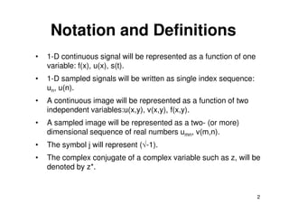
This document provides definitions and notations for 2-D systems and matrices. It defines how continuous and sampled 2-D signals like images are represented. It introduces some common 2-D functions used in signal processing like the Dirac delta, rectangle, and sinc functions. It describes how 2-D linear systems can be represented by matrices and discusses properties of the 2-D Fourier transform including the frequency response and eigenfunctions. It also introduces concepts of Toeplitz and circulant matrices and provides an example of convolving periodic sequences using circulant matrices. Finally, it defines orthogonal and unitary matrices.

1. 02. 2-D Systems and
Matrix
Tati R. Mengko

2. Notation and Definitions
• 1-D continuous signal will be represented as a function of one
variable: f(x), u(x), s(t).
• 1-D sampled signals will be written as single index sequence:
un, u(n).
• A continuous image will be represented as a function of two
independent variables:u(x,y), v(x,y), f(x,y).
• A sampled image will be represented as a two- (or more)
dimensional sequence of real numbers umn, v(m,n).
• The symbol j will represent (√-1).
• The complex conjugate of a complex variable such as z, will be
denoted by z*.
2

3. Some Special Functions
• Dirac Delta:
δ ( x, y ) = δ ( x ) δ ( y )
∞ ∞
∫ ∫ f ( x ', y ')δ ( x − x ', y − y ') dx ' dy ' = f ( x, y )
−∞ −∞
ε ε
lim ∫ ∫ δ ( x, y )dxdy = 1
ε ε ε
→0 − −
• Kronecker Delta:
δ ( m, n ) = δ ( m ) δ ( n )
∞ ∞
x ( m, n ) = ∑ ∑ x ( m ', n ')δ ( m − m ', n − n ')
m ' =−∞ n ' =∞
∞ ∞
∑ ∑ δ ( m, n ) = 1
m =−∞ n =∞
3

4. Some Special Functions
• Rectangle
1 x ≤ 1 2 dan y ≤
 1
rect ( x, y ) = 
2
0 lainnya

• Sinc 2-D
sin π x sin π y
sinc ( x, y ) =
πx πy
• Comb
∞ ∞
comb ( k , l ) = ∑ ∑ δ ( k − k ', l − l ')
k ' =−∞ l ' =∞
4

5. 2-D Linear System
x(m,n) y(m,n) = H [x(m,n)]
y(m,n)
H [.]
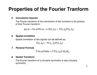
• Linear system criterion:
H [a1x1(m,n) + a2x2(m,n)] = a1H [x1(m,n)] + a2H [x2(m,n)]
= a1 y1(m,n) + a2 y2(m,n)
• Impulse response:
System response (output) given a delta kronecker input:
h(m,n; m’,n’) ≡ H [δ(m - m’, n - n’)]
– PSF (point spread function) → impulse response whose inputs
and outputs represent a positive quantity, such as intensity.
5

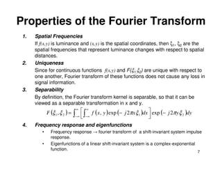
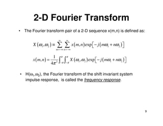
6. The Fourier Transform
• 2-D Fourier/ Inverse Fourier Transform Formulations:
∞ ∞
F (ξ1 ,ξ 2 ) = ∫ ∫ f ( x, y ) exp  − j 2π ( xξ1 + yξ 2 )  dxdy
 
−∞ −∞
∞ ∞
f ( x, y ) = ∫ ∫ F (ξ1 ,ξ 2 ) exp  j 2π ( xξ1 + yξ 2 )  dξ1dξ 2
 
−∞ −∞
f(x,y) F(ξ1, ξ2)
δ(x,y) 1
δ(x ± x0, y ± y0) exp(±j2πx0ξ1). exp(±j2πy0ξ2)
exp(±j2πx0η1). exp(±j2πy0 η2) δ(ξ1 -+ η1, ξ2 -+ η2)
exp[-π(x2 + y2 )] exp[-π(ξ12 + ξ22 )]
rect(x, y) sinc(ξ1, ξ2)
tri(x, y) sinc2(ξ1, ξ2)
comb(x, y) comb(ξ1, ξ2)
6

7. Properties of the Fourier Transform
1. Spatial Frequencies
If f(x,y) is luminance and (x,y) is the spatial coordinates, then ξ1, ξ2 are the
spatial frequencies that represent luminance changes with respect to spatial
distances.
2. Uniqueness
Since for continuous functions f(x,y) and F(ξ1,ξ2) are unique with respect to
one another, Fourier transform of these functions does not cause any loss in
signal information.
3. Separability
By definition, the Fourier transform kernel is separable, so that it can be
viewed as a separable transformation in x and y.
F (ξ 1 , ξ 2 ) =
∞
 ∞ f ( x , y ) exp (− j 2π x ξ )dx  exp (− j 2π y ξ )dy
∫− ∞  ∫− ∞
 1 
 2
4. Frequency response and eigenfunctions
• Frequency response → fourier transform of a shift-invariant system impulse
response.
• Eigenfunctions of a linear shift-invariant system is a complex-exponential
function.
7

8. Properties of the Fourier Tranform
5. Convolution theorem
The Fourier transform of the convolution of two functions is the product
of their Fourier transform:
g(x,y) = h(x,y)⊗f(x,y) ⇔ G(ξ1,ξ2) = H(ξ1,ξ2)F(ξ1,ξ2)
6. Spatial correlation
Spatial correlation of two signals can be defined as:
C(ξ1,ξ2) = H(-ξ1,-ξ2)F(ξ1,ξ2)
7. Parseval Formula
∫∫ |f(x,y)|2dxdy = ∫∫ |F(ξ1,ξ2)|2 dξ1dξ2
8. Hankel Transform
The Fourier transform of a circularly symmetric is also circularly
symmetric.
8

9. 2-D Fourier Transform
• The Fourier transform pair of a 2-D sequence x(m,n) is defined as:
∞ ∞
X (ω1 ,ω 2 ) ≡ ∑ ∑ x ( m, n ) exp − j ( mω
m =−∞ n =−∞
 1 + nω 2 ) 

1 π π
x ( m, n ) = ∫ π ∫ π X (ω ,ω ) exp − j ( mω
 + nω 2 ) 

4π 2 1 2 1
− −
• H(ω1,ω2), the Fourier transform of the shift invariant system
impulse response, is called the frequency response.
9

10. Matrix Theory
• One- and two-dimensional sequence will be represented by vectors
and matrices.
 u (1)   a (1,1) a (1, 2 ) ... a (1, N ) 
 u (2 )  a (2 ,1) a (2 , 2 ) ... a (2 , N ) 
u ≡ {u (n )} =   A ≡ {a (m , n )} =  
 ...   ... ... ... ... 
   
 u (n )  a (M ,1) a (M , 2 ) ... a (M , N )
• Transpose: AT = {a(m,n)}T = {a(n,m)}
• Transposition and Conjugation Rules
1. A*T = [AT]*
2. [AB] = BTAT
3. [A-1]T = [AT]-1
4. [AB]* = A*B*
10

11. Toeplitz and Circulant Matrices
• A Toeplitz matrix T is a matrix that has constant elements along the
main diagonal and the subdiagonals.
• A matrix C is called circulant if each of its rows (or columns) is a
circular shift of the previous row (or columns)
 t0 t −1 ... ... t − N +1   c0 c1 c2 ... c N −1 
 t t0 t −1 ... t− N +2  c c0 c1 ... cN −2 
 1   N −1 
T =  t2 ... ...  C =  ... ... ... ... ... 
   
 ... ... ... ... ...   c2 ... ... ... ... 

 t N −1 ... t2 t1 t0    c1
 c2 ... c N −1 cN  
• Note that C is also Toeplitz and:
c(m,n) = c((m,n) modulo N)
11

12. Example
• A LSI (linear shift invariant) system  y (− 1) − 1 0 0 0 0 
h(n)=n, -1≤n≤1 with input x(n) which is  y (0 )   0 − 1 0 0 0   x(0 )
zero outside 0≤n≤4, is given by the    
 
 y (1)   1 0 − 1 0 0   x(1) 
convolution:   =  0 1 0 − 1 0   x(2 )
 y (2 )   
 
y(n) = h(n)⊗x(n)= Σ0~4h(n-k)x(k).  y (3)   0 0 1 0 − 1  x(3)
 y (4 )   
   0 0 0 1 0   x(4 )
 
 y (5)   0 0 0 0 1 
   
• If two convolving sequences are
periodic, then their convolution is also
periodic and can be represented as  y (0 )  3 2 1 0   x (0 )
 y (1)   0 3 2 1   x (1) 
y(n) = Σ0~(N-1) h(n-k)x(k), 0 ≤n≤N-1  =  
 y (2 )  1 0 3 2   x (2 )
where h(-n) = h(N-4) and N is the period.  y (3 )  2
   1 0
 
3   x (3 )
Let N=4 and h(n)=n+3 (modulo 4). In
vector notation this gives
12

13. Orthogonal and Unitary Matrices
• An orthogonal matrix is such that its inverse is equal to
its transpose, A is orthogonal if :
A-1 = AT or ATA = AAT = I
• A matrix is called unitary if its inverse is equal to its
conjugate transpose:
A-1 = A*T or AA*T = A*TA = I
• Orthogonality and unitary characteristics indicate the
transform energy conservation properties.
13

14. Thank you
14