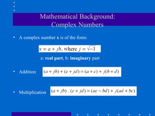
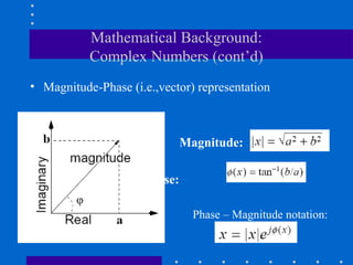
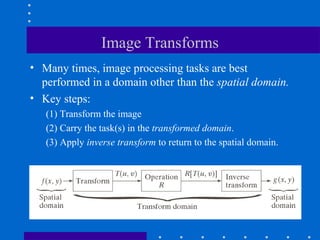
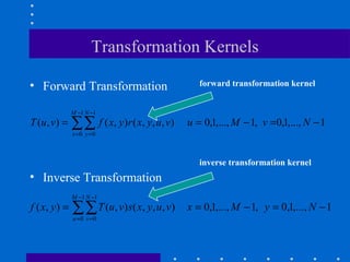
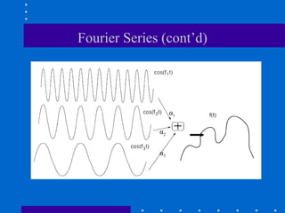
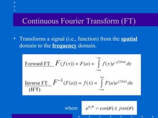
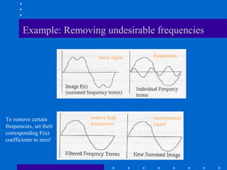
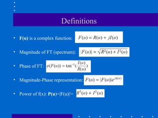
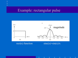
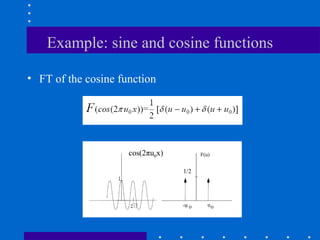
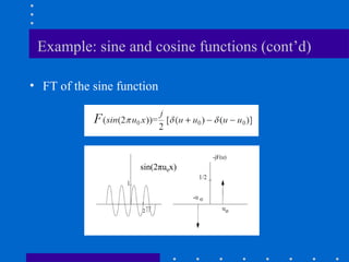
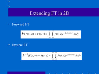
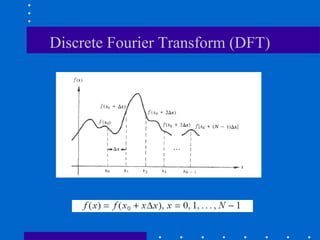
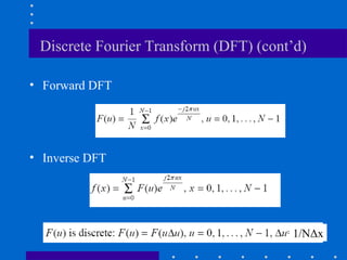
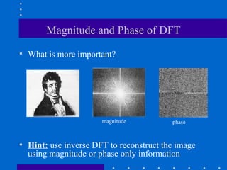
The Fourier transform decomposes a signal into its constituent frequencies, representing it in the frequency domain rather than the spatial domain, which can make certain operations and analyses easier to perform; it has both magnitude and phase components that provide information about the frequency content and relative phases of the signal. The discrete Fourier transform (DFT) is a sampled version of the continuous Fourier transform that is useful for digital signal and image processing applications.

1. Fourier Transform
Naveen Sihag

2. Mathematical Background:
Complex Numbers
• A complex number x is of the form:
a: real part, b: imaginary part
• Addition
• Multiplication

3. Mathematical Background:
Complex Numbers (cont’d)
• Magnitude-Phase (i.e.,vector) representation
Magnitude:
Phase:
φ
Phase – Magnitude notation:

4. Mathematical Background:
Complex Numbers (cont’d)
• Multiplication using magnitude-phase representation
• Complex conjugate
• Properties

5. Mathematical Background:
Complex Numbers (cont’d)
• Euler’s formula
• Properties
j

6. Mathematical Background:
Sine and Cosine Functions
• Periodic functions
• General form of sine and cosine functions:

7. Mathematical Background:
Sine and Cosine Functions
Special case: A=1, b=0, α=1
π
π

8. Mathematical Background:
Sine and Cosine Functions (cont’d)
• Shifting or translating the sine function by a const b
Note: cosine is a shifted sine function:
π
cos(t ) = sin(t + )
2

9. Mathematical Background:
Sine and Cosine Functions (cont’d)
• Changing the amplitude A

10. Mathematical Background:
Sine and Cosine Functions (cont’d)
• Changing the period T=2π/|α|
consider A=1, b=0: y=cos(αt)
α =4
period 2π/4=π/2
shorter period
higher frequency
(i.e., oscillates faster)
Frequency is defined as f=1/T
Alternative notation: sin(αt)=sin(2πt/T)=sin(2πft)

11. Image Transforms
• Many times, image processing tasks are best
performed in a domain other than the spatial domain.
• Key steps:
(1) Transform the image
(2) Carry the task(s) in the transformed domain.
(3) Apply inverse transform to return to the spatial domain.

12. Transformation Kernels
• Forward Transformation forward transformation kernel
M −1 N −1
T (u , v) = ∑∑ f ( x, y)r ( x, y, u, v)
x =0 y =0
u = 0,1,..., M − 1, v =0,1,..., N − 1
inverse transformation kernel
• Inverse Transformation
M −1 N −1
f ( x, y ) = ∑∑ T (u, v)s( x, y, u, v)
u =0 v =0
x = 0,1,..., M − 1, y = 0,1,..., N − 1

13. Kernel Properties
• A kernel is said to be separable if:
r ( x, y, u, v) = r1 ( x, u )r2 ( y, v)
• A kernel is said to be symmetric if:
r ( x, y, u , v) = r1 ( x, u )r1 ( y, v)

14. Notation
• Continuous Fourier Transform (FT)
• Discrete Fourier Transform (DFT)
• Fast Fourier Transform (FFT)

15. Fourier Series Theorem
• Any periodic function can be expressed as a weighted
sum (infinite) of sine and cosine functions of varying
frequency:
is called the “fundamental frequency”

16. Fourier Series (cont’d)
α1
α2
α3

17. Continuous Fourier Transform (FT)
• Transforms a signal (i.e., function) from the spatial
domain to the frequency domain.
(IFT)
where

18. Why is FT Useful?
• Easier to remove undesirable frequencies.
• Faster perform certain operations in the frequency
domain than in the spatial domain.

19. Example: Removing undesirable frequencies
noisy signal frequencies
To remove certain remove high reconstructed
frequencies signal
frequencies, set their
corresponding F(u)
coefficients to zero!

20. How do frequencies show up in an image?
• Low frequencies correspond to slowly varying
information (e.g., continuous surface).
• High frequencies correspond to quickly varying
information (e.g., edges)
Original Image Low-passed

21. Example of noise reduction using FT

22. Frequency Filtering Steps
1. Take the FT of f(x):
2. Remove undesired frequencies:
3. Convert back to a signal:
We’ll talk more about this later .....

23. Definitions
• F(u) is a complex function:
• Magnitude of FT (spectrum):
• Phase of FT:
• Magnitude-Phase representation:
• Power of f(x): P(u)=|F(u)|2=

24. Example: rectangular pulse
magnitude
rect(x) function sinc(x)=sin(x)/x

25. Example: impulse or “delta” function
• Definition of delta function:
• Properties:

26. Example: impulse or “delta” function (cont’d)
• FT of delta function:
1
x
u

27. Example: spatial/frequency shifts
f ( x) ↔ F (u ), then
Special Cases:
− j 2πux0
(1) f ( x − x0 ) ↔ e − j 2πux0
F (u ) δ ( x − x0 ) ↔ e
j 2πu0 x
( 2) f ( x ) e j 2πu0 x
↔ F (u − u 0 ) e ↔ δ (u − u 0 )

28. Example: sine and cosine functions
• FT of the cosine function
cos(2πu0x) F(u)
1/2

29. Example: sine and cosine functions (cont’d)
• FT of the sine function
-jF(u)
sin(2πu0x)

30. Extending FT in 2D
• Forward FT
• Inverse FT

31. Example: 2D rectangle function
• FT of 2D rectangle function
2D sinc()

32. Discrete Fourier Transform (DFT)

33. Discrete Fourier Transform (DFT) (cont’d)
• Forward DFT
• Inverse DFT
1/NΔx

34. Example

35. Extending DFT to 2D
• Assume that f(x,y) is M x N.
• Forward DFT
• Inverse DFT:

36. Extending DFT to 2D (cont’d)
• Special case: f(x,y) is N x N.
• Forward DFT
u,v = 0,1,2, …, N-1
• Inverse DFT
x,y = 0,1,2, …, N-1

37. Visualizing DFT
• Typically, we visualize |F(u,v)|
• The dynamic range of |F(u,v)| is typically very large
• Apply streching: (c is const)
original image before scaling after scaling

38. DFT Properties: (1) Separability
• The 2D DFT can be computed using 1D transforms only:
Forward DFT:
Inverse DFT:
kernel is ux + vy ux vy
− j 2π ( ) − j 2 π ( ) − j 2π ( )
separable: e N
=e N
e N

39. DFT Properties: (1) Separability (cont’d)
• Rewrite F(u,v) as follows:
• Let’s set:
• Then:

40. DFT Properties: (1) Separability (cont’d)
• How can we compute F(x,v)?
)
N x DFT of rows of f(x,y)
• How can we compute F(u,v)?
DFT of cols of F(x,v)

41. DFT Properties: (1) Separability (cont’d)

42. DFT Properties: (2) Periodicity
• The DFT and its inverse are periodic with period N

43. DFT Properties: (3) Symmetry
• If f(x,y) is real, then
(see Table 4.1 for more properties)

44. DFT Properties: (4) Translation
f(x,y) F(u,v)
• Translation is spatial domain:
• Translation is frequency domain:
)
N

45. DFT Properties: (4) Translation (cont’d)
• Warning: to show a full period, we need to translate
the origin of the transform at u=N/2 (or at (N/2,N/2)
in 2D)
|F(u)|
|F(u-N/2)|

46. DFT Properties: (4) Translation (cont’d)
• To move F(u,v) at (N/2, N/2), take
Using )
N

47. DFT Properties: (4) Translation (cont’d)
no translation after translation

48. DFT Properties: (5) Rotation
• Rotating f(x,y) by θ rotates F(u,v) by θ

49. DFT Properties: (6) Addition/Multiplication
but …

50. DFT Properties: (7) Scale

51. DFT Properties: (8) Average value
Average:
F(u,v) at u=0, v=0:
So:

52. Magnitude and Phase of DFT
• What is more important?
magnitude phase
• Hint: use inverse DFT to reconstruct the image
using magnitude or phase only information

53. Magnitude and Phase of DFT (cont’d)
Reconstructed image using
magnitude only
(i.e., magnitude determines the
contribution of each component!)
Reconstructed image using
phase only
(i.e., phase determines
which components are present!)

54. Magnitude and Phase of DFT (cont’d)