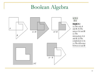
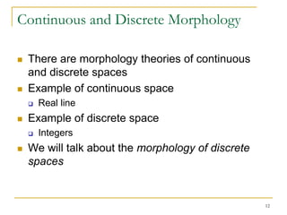
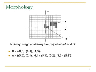
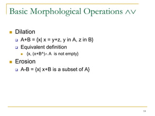
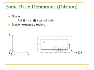
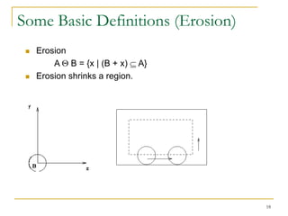
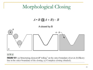
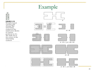
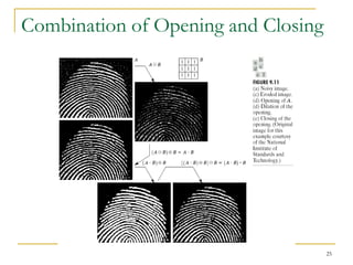
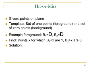
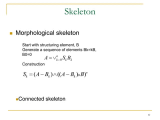
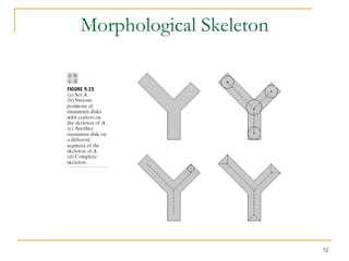
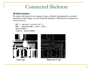
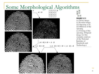
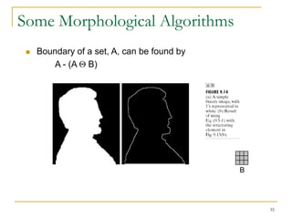
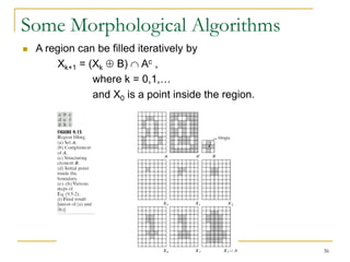
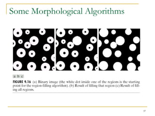
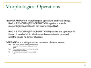
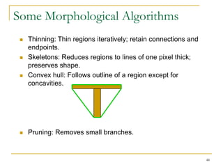
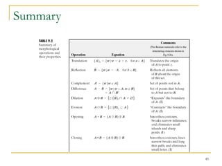
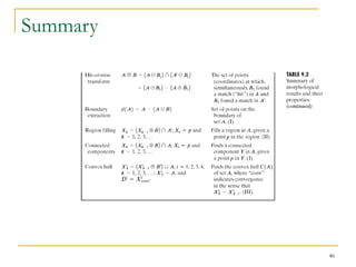
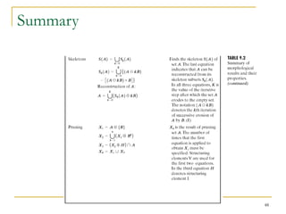
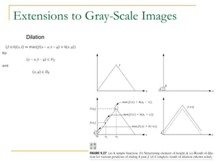
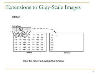
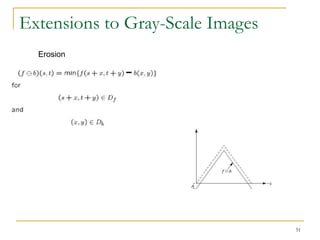
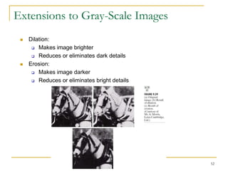
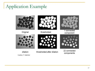
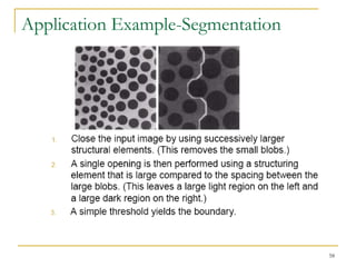
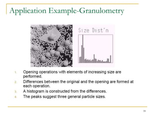
The document discusses morphological image operations and mathematical morphology. It provides examples of basic morphological operations like dilation, erosion, opening and closing. It also discusses morphological algorithms for tasks like boundary extraction, region filling, connected component extraction, skeletonization, and using morphological operations for applications like detecting foreign objects. The key concepts covered are binary morphological operations, connectivity in images, and algorithms for thinning, boundary detection, and segmentation.

1. Morphological Image Operation

2.  Download di http://rumah-belajar.org
2

3. Mathematical Morphology
 Mathematical morphology is a powerful
methodology which was initiated in the late
1960s by G.Matheron and J.Serra at the
Fontainebleau School of Mines in France.
 nowadays it offers many theoretic and
algorithmic tools inspiring the development of
research in the fields of signal
processing, image processing, machine
vision, and pattern recognition.
3

4. Morphological Operations -1
The four most basic operations in mathematical
morphology are dilation, erosion, opening and Closing:
4

5. Morphological Image Processing
 Boolean algebra
 Dilation and erosion
 Opening and closing
 Hit-or-miss
 Basic algorithms
 Extension to gray-scale
5

6. Examples of Boolean Algebra
 Switching algebra
 S = {0, 1}
 Finite Boolean algebras
 Example: S = {(0, 0), (0, 1), (1, 0), (1, 1)}
 (a1, a2)’ = (a’1, a’2)
 (0, 1) (1, 0) = (0, 0)
 Set unions/intersections
 Union is like
 Intersection is like
 Empty set is like 0
 There is no 1 (universal set)
6

7. Review: Boolean Algebra
 A Boolean algebra is a set with at least two
elements, three operations (and , or , not ‘) and two
special elements (0, 1) that have the following
properties.
 A B is an element of the set. This function is defined for all
elements A and B in the set. It is symmetric (A B = B A)
 A B has the same properties
 A’ is defined for all elements in the set.
 A A’=0, A A’=1
 The operations and + are distributive.
 A (B C)=(A B) (A C)
 A (B C)=(A B) (A C)
 0 and 1 are identities, in the following sense
 0 A=A
 1 A=A
7

8. Some Basic Definitions
 Let A and B be sets with components a=(a1,a2) and
b=(b1,b2), respectively.
 The translation of A by x=(x1,x2) is
A + x = {c | c = a + x, for a A}
 The reflection of A is
Ar = {x | x = -a for a A}
 The complement of A is
Ac = {x | x A}
 The union of A and B is
A B = {x | x A or x B }
 The intersection of A and B is
A B = {x | x A and x B }
8

9. Some Basic Definitions
 The difference of A and B is.
A – B = A Bc = {x | x A and x B}
 A and B are said to be disjoint or mutually exclusive if they
have no common elements.
 If every element of a set A is also an element of another set
B, then A is said to be a subset of B.
9

10. Additional Operations
 Elements of set: points
 Points are integers (1-D discrete space)
 Points are 2-D vectors with integer components (2-D
discrete space)
 Operations
 Addition (vector addition)
 Reflection (multiply by -1)
 Integer multiplication
 A set of points can be translated or reflected
 S+x = x+S (new set consists of all points of
S, translated by x)
 S^ is the set reflected through the origin
10

11. Boolean Algebra
11

12. Continuous and Discrete Morphology
 There are morphology theories of continuous
and discrete spaces
 Example of continuous space
 Real line
 Example of discrete space
 Integers
 We will talk about the morphology of discrete
spaces
12

13. Morphology
A binary image containing two object sets A and B
 B = {(0,0), (0,1), (1,0)}
 A = {(5,0), (3,1), (4,1), (5,1), (3,2), (4,2), (5,2)}
13

14. Basic Morphological Operations
 Dilation
 A+B = {x| x = y+z, y in A, z in B}
 Equivalent definition
 {x, (x+B^) A is not empty}
 Erosion
 A-B = {x| x+B is a subset of A}
14

15. Some Basic Definitions (Dilation)
 Dilation
A B = {x | (B + x) A }
 Dilation expands a region.
15

16. Example (1)
16

17. More Examples (2)
17

18. Some Basic Definitions (Erosion)
 Erosion
A B = {x | (B + x) A}
 Erosion shrinks a region.
18

19. More Examples (3)
19

20. Some Basic Definitions (opening)
 Opening is erosion followed by dilation:
A B = (A B) B
 Opening smoothes regions, removes spurs, breaks narrow
lines.
20

21. Morphological Opening
A oB @(A B) B
A opened by B
21

22. Some Basic Definitions (closing)
 Closing is dilation followed by erosion:
A B = (A B) B
 Closing fills narrow gaps and holes in a region.
22

23. Morphological Closing
A • B @(A B) B
A closed by B
23

24. Example
24

25. Combination of Opening and Closing
25

26. Hit-or-Miss
 Given: points on plane
 Template: Set of one points (foreground) and set
of zero points (background)
 Example foreground: B1=D, B2=D
 Find: Points x for which B1+x are 1, B2+x are 0
 Solution:
26

27. Exp:
27

28. Boundary Extraction
(A) A (A B)'
28

29. Region Filling
Xk (Xk 1 B) A'
•Start with point in region A.
Keep expanding by
dilation, using points in region A
only.
29

30. Extraction of Connected Component
Xk (Xk 1 B) A
 Start with point
on object. Keep
adding points
30

31. Skeleton
 Morphological skeleton
Start with structuring element, B
Generate a sequence of elements Bk=kB,
B0=0 n
A k 0 Sk Bk
Construction
Sk (A Bk ) ((A Bk ) B)'
Connected skeleton
31

32. Morphological Skeleton
32

33. Connected Skeleton
33

34. Some Morphological Algorithms
34

35. Some Morphological Algorithms
 Boundary of a set, A, can be found by
A - (A B)
B
35

36. Some Morphological Algorithms
 A region can be filled iteratively by
Xk+1 = (Xk B) Ac ,
where k = 0,1,…
and X0 is a point inside the region.
36

37. Some Morphological Algorithms
37

38. Morphological Operations
BWMORPH Perform morphological operations on binary image.
BW2 = BWMORPH(BW1,OPERATION) applies a specific
morphological operation to the binary image BW1.
BW2 = BWMORPH(BW1,OPERATION,N) applies the operation N
times. N can be Inf, in which case the operation is repeated
until the image no longer changes.
OPERATION is a string that can have one of these values:
'skel' With N = Inf, remove pixels on the boundaries
of objects without allowing objects to break
apart
'spur' Remove end points of lines without removing
small objects completely.
'fill' Fill isolated interior pixels (0's surrounded by
1's)
...
38

39. Morphological Operations
BW1 = imread('circbw.tif');
BW2 = bwmorph(BW1,'skel',Inf);
imshow(BW1);
figure, imshow(BW2);
39

40. Morphological Operations
BW1 = imread('circbw.tif');
BW2 = bwperim(BW1);
imshow(BW1);
figure, imshow(BW2)
40

41. Morphological Operations
Pixel Connectivity
Connectivity defines which pixels are connected to other pixels. A set of
pixels in a binary image that form a connected group is called an object
or a connected component.
4-connected 8-connected
41

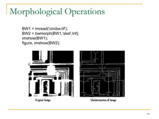
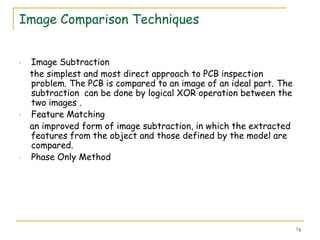
42. Morphological Operations
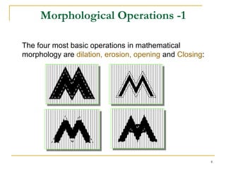
BW = [0 0 0 0 0 0 0 0;
0 1 1 0 0 1 1 1;
0 1 1 0 0 0 1 1; X = bwlabel(BW,4);
0 1 1 0 0 0 0 0; RGB = label2rgb(X, @jet, 'k');
0 0 0 1 1 0 0 0; imshow(RGB,'notruesize')
0 0 0 1 1 0 0 0;
0 0 0 1 1 0 0 0;
0 0 0 0 0 0 0 0];
X = bwlabel(BW,4)
X = 0 0 0 0 0 0 0 0
0 1 1 0 0 3 3 3
0 1 1 0 0 0 3 3
0 1 1 0 0 0 0 0
0 0 0 2 2 0 0 0
0 0 0 2 2 0 0 0
0 0 0 2 2 0 0 0
0 0 0 0 0 0 0 0
42

43. Some Morphological Algorithms
Application example: Using
connected components to detect
foreign objects in packaged food.
There are four objects with
significant size!
43

44. Some Morphological Algorithms
 Thinning: Thin regions iteratively; retain connections and
endpoints.
 Skeletons: Reduces regions to lines of one pixel thick;
preserves shape.
 Convex hull: Follows outline of a region except for
concavities.
 Pruning: Removes small branches.
44

45. Summary
45

46. Summary
46

47. Summary
47

48. Summary
48

49. Extensions to Gray-Scale Images
Dilation
49

50. Extensions to Gray-Scale Images
Dilation
Take the maximum within the window.
50

51. Extensions to Gray-Scale Images
Erosion
51

52. Extensions to Gray-Scale Images
 Dilation:
 Makes image brighter
 Reduces or eliminates dark details
 Erosion:
 Makes image darker
 Reduces or eliminates bright details
52

53. Extensions to Gray-Scale Images
53

54. Extensions to Gray-Scale Images
Opening: Narrow bright areas are reduced.
Closing: Narrow dark areas are reduced.
54

55. Extensions to Gray-Scale Images
56

56. Application Example
57

57. Application Example-Segmentation
58

58. Application Example-Granulometry
59

59. Morphological Reconstruction (exp.algo)
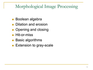
 Algorithm for binary reconstruction:
1. M = V o K , where K is any SE.
2. T = M,
3. M= M Ki , where i=4 or i=8,
4. M = M∩ V, [Take only those pixels from M that are also in V .]
5. if M T then go to 2,
6. else stop;
Original (V) Opened (M) Reconstructed (T)
60

60. Application in 2D Image Processing
Character Extraction-1
Character Extraction From Cover Image (Source)
61

61. Application in 2D Image Processing
Character Extraction-2
Character Extraction From Cover Image (Results)
62

62. Application in 2D Image Processing
Character Extraction-3
Morning Noon
Afternoon Evening
63

63. Application in 2D Image Processing
Character Extraction-4
Morning Noon
Afternoon Evening
64

64. Application in 3D Image Processing
Organs Extraction-1
slice20 slice25 slice30
slice25 slice30 65
slice20

65. Application in 3D Image Processing
Organs Extraction-2
Top View Back View
66

66. Application in 3D Image Processing
Organs Extraction-3
67

67. Application in 3D Image Processing
Organs Extraction-4
Segmented heart beating cycle
68

68. Application in 3D Image Processing
Organs Extraction-5
Kidney with Bones Kidney with Vessels
69

69. Brain View snapshot-3
--Registration tool kit
Features:
1. Cut plane in 3D
2. Work in 2 data sets
3. 2D and 3D view
4. Registration methods:
• LandMark
• ThinPlateSpline
• GridTransform
• MutualInformation
70

70. Brain View snapshot-4
--Segmenation tool kit
Features:
1. Cut plane in 3D
2. Work in 2 data sets
3. 2D and 3D view
4. Segmenation
methods:
• Morphology
• Snake
• Level Set
• Watershed
71

71. Research Plan-1
 Medical Image Analysis
--- Segmentation and Registration
 More efforts address on Ultrasound Image (2D, 3D)
Segmented baby face from US
2D Segmentation using GDM 72
Real time US, MR integration for IGS

72. 73

73. Image Comparison Techniques
• Image Subtraction
the simplest and most direct approach to PCB inspection
problem. The PCB is compared to an image of an ideal part. The
subtraction can be done by logical XOR operation between the
two images .
• Feature Matching
an improved form of image subtraction, in which the extracted
features from the object and those defined by the model are
compared.
• Phase Only Method
74

74. Example PCB and Mask
75

75. Result
short
spur
dirt
open
mousebite
pinhole
76

76. Question
77