The document discusses various image transforms. It begins by explaining why transforms are used, such as for fast computation and obtaining conceptual insights. It then introduces image transforms as unitary matrices that represent images using a discrete set of basis images. It proceeds to describe one-dimensional orthogonal and unitary transforms using matrices. It also discusses separable two-dimensional transforms and provides properties of unitary transforms such as energy conservation. Specific transforms discussed in more detail include the discrete Fourier transform, discrete cosine transform, discrete sine transform, and Hadamard transform.

1. Image Transforms

2. Why Do Transforms?
 Fast computation
 E.g., convolution vs. multiplication for filter with
wide support
 Conceptual insights for various image processing
 E.g., spatial frequency info. (smooth, moderate
change, fast change, etc.)
 Obtain transformed data as measurement
 E.g., blurred images, radiology images (medical
and astrophysics)
 Often need inverse transform
 May need to get assistance from other transforms
 For efficient storage and transmission
 Pick a few “representatives” (basis)
 Just store/send the “contribution” from each basis

3. Introduction
 Image transforms are a class of
unitary matrices used for
representing images.
 An image can be expanded in terms
of a discrete set of basis arrays called
basis images.
 The basis images can be generated
by unitary matrices.

4. One dimensional orthogonal and unitary
transforms
 For a 1-D sequence represented
as a vector u of size N, a unitary transformation
is written as
{ ( ),0 1}u n n N  
1
0
( ) ( , ) ( ) , 0 1
N
n
v k a k n u n k N


    v = Au

5. 1
*
0
( ) ( ) ( , ) , 0 1
N
k
u n v k a k n n N


   
*T
u = A v
v(k) is the series representation of the sequence u(n).
The columns of A*T, that is, the vectors
are called the basis vectors of A.
*
{ ( , ), 0 1}T
a k n n N   *
ka
One dimensional orthogonal and unitary
transforms

6. Two-dimensional orthogonal and
unitary transforms
 A general orthogonal series expansion for an N x
N image u(m,n) is a pair of transformations of
the form
1 1
,
0 0
( , ) ( , ) ( , )
N N
k l
m n
y k l x m n a m n
 
 
 
1 1
*
,
0 0
( , ) ( , ) ( , )
N N
k l
k l
x m n y k l a m n
 
 
 
 ,where ( , ) ,k la m n called an image transform, is a set of complete
orthonormal discrete basis functions.

7. Separable unitary transforms
 Complexity : O(N4)
 Reduced to O(N3) when transform is separable i.e.
ak,l(m,n) = ak(m) bl(n) =a(k,m)b(l,n) where
{a(k,m), k=0,…,N-1},{b(l,n), l=0,…,N-1}
are 1-D complete orthonormal sets of basis vectors.

8. Separable unitary transforms
 A={a(k,m)} and B={b(l,n)} are unitary
matrices i.e. AA*T = ATA* = I.
 If B is same as A
1 1
0 0
( , ) ( , ) ( , ) ( , )
N N
m n
y k l a k m x m n a l n
 
 
   T
Y AXA
1 1
* * *
0 0
( , ) ( , ) ( , ) ( , )
N N
T
k l
x m n a k m y k l a l n
 
 
  *
X = A YA

9. Basis Images
 Let denote the kth column of . Define the matrices
then
*
ka *T
A
* * *T
k,l k lA = a a
1 1
0 0
( , )
( , ) ,
N N
k l
y k l
y k l
 
 


 *
k,l
*
k,l
X A
X A
, 0,..., 1k l N *
k,lA
The above equation expresses image X as a linear
combination of the N2 matrices , called
the basis images.

10. 8x8 Basis images for discrete cosine transform.

11. Example
 Consider an orthogonal matrix A and image X
1 11
1 12
A
 
   







43
21
X
1 1 1 2 1 1 5 11
1 1 3 4 1 1 2 02
       
                 
T
Y = AXA
To obtain basis images, we find the outer product of the
columns of A*T
* *
0,1 1,0
1 11
1 12
T
A A
 
   
*
1,1
1 11
1 12
A
 
   
 *
0,0
1 1 11 1
1 1
1 1 12 2
A
   
    
   
The inverse transformation gives
1 1 5 1 1 1 1 21
1 1 2 0 1 1 3 42
     
             
*T *
X = A YA

12. Properties of Unitary Transforms
Energy Conservation
In unitary transformation, y = Ax and ||y||2 = ||x||2
1 1
2 2
0 0
( ) ( )
N N
k n
y k x n
 
 
    
2 2*T *T *T *T
y y y = x A Ax = x x x
Proof:
This means every unitary transformation is simply a rotation
of the vector x in the N-dimensional vector space.
Alternatively, a unitary transformation is rotation of the basis
coordinates and the components of y are the projections of x
on the new basis.

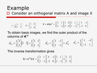
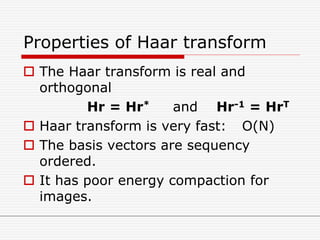
13. Properties of Unitary Transforms
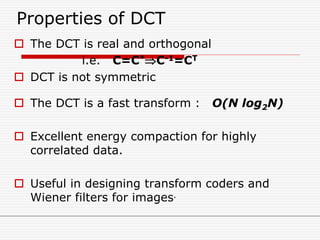
 Energy compaction
 Unitary transforms pack a large fraction of the
average energy of the image into a relatively
few components of the transform coefficients.
i.e. many of the transform coefficients contain
very little energy.
 Decorrelation
 When the input vector elements are highly
correlated, the transform coefficients tend to be
uncorrelated.
 Covariance matrix E[ ( y – E(y) ) ( y – E(y) )*T ].
 small correlation implies small off-diagonal terms.

14. 1-D Discrete Fourier Transform
1
0
1
( ) ( ) , 0,..., -1
N
nk
N
n
y k x n W k N
N


 
2
expN
j
W
N
 
  
 
The discrete Fourier transform (DFT) of a sequence {u(n), n=0,…,N-1} is
defined as
where
The inverse transform is given by
1
0
1
( ) ( ) , 0,..., -1
N
nk
N
k
x n y k W n N
N



 
The NxN unitary DFT matrix F is given by
1
, 0 , 1nk
NF W k n N
N
 
    
 

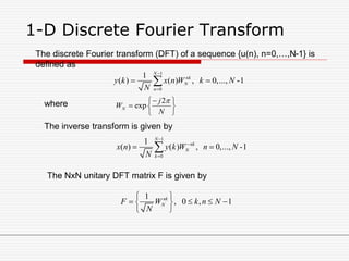
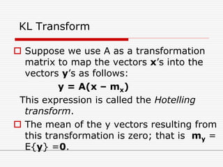
15. DFT Properties
 Circular shift u(n-l)c = x[(n-l)mod N]
 The DFT and unitary DFT matrices are
symmetric i.e. F-1 = F*
 DFT of length N can be implemented by a fast
algorithm in O(N log2N) operations.
 DFT of a real sequence {x(n), n=0,…,N-1} is
conjugate symmetric about N/2.
i.e. y*(N-k) = y(k)

16. The Two dimensional DFT
1 1
0 0
1
( , ) ( , ) , 0 , -1
N N
km ln
N N
m n
y k l x m n W W k l N
N
 
 
  
1 1
0 0
1
( , ) ( , ) , 0 , -1
N N
km ln
N N
k l
x m n y k l W W m n N
N
 
 
 
  
The 2-D DFT of an N x N image {x(m,n)} is a separable
transform defined as
Y = FXF * *
X = F YF
The inverse transform is
In matrix notation &

17. Properties of the 2-D DFT
 Symmetric,
unitary.
 Periodic
 Conjugate
Symmetry
 Fast transform
 Basis Images
T -1
  * *
F F*
F F, F F =
( , ) ( , ), ,
( , ) ( , ), ,
y k N l N y k l k l
x m N n N x m n m n
   
   
*
( , ) ( , ), 0 , 1y k l y N k N l k l N     
 * ( )
,
1
, 0 , 1 , 0 , 1T km ln
k l k l NA W m n N k l N
N
 
         
O(N2log2N)

18. 2-D pulse DFT
Square Pulse
2D sinc function

19. FT is Shift Invariant
After shifting:
• Magnitude stay constant
• Phase changes

20. Rotation
• FT of a rotated image also
rotates

21. The Cosine Transform (DCT)
1
0
(2 1)
( ) ( ) ( )cos , 0 1
2
N
n
n k
y k k x n k N
N





   
1
, 0,0 1
( , )
2 (2 1)
cos , 1 1,0 1
2
k n N
N
C k n
n k
k N n N
N N


   

 
      

1
0
(2 1)
( ) ( ) ( )cos , 0 1
2
N
k
n k
x n k y k n N
N





   
The N x N cosine transform matrix C={c(k,n)}, also known
as discrete cosine transform (DCT), is defined as
1 2
(0) , ( ) = for 1 1
N
k k N
N
    
The 1-D DCT of a sequence {x(n), 0 ≤ n ≤ N-1} is defined as
The inverse transformation is given by
where

22. Properties of DCT
 The DCT is real and orthogonal
i.e. C=C*C-1=CT
 DCT is not symmetric
 The DCT is a fast transform : O(N log2N)
 Excellent energy compaction for highly
correlated data.
 Useful in designing transform coders and
Wiener filters for images.

23. 2-D DCT
(2 1) (2 1)
( , , , ) ( ) ( )cos cos
2 2
m k n l
C m n k l k l
N N
 
 
 

1
0
( )
2
1 1
k
N
k
k N
N




 
   
The 2-D DCT Kernel is given by
where
Similarly for ( )l

24. DCT example
a) Original image b) DCT image

25. The Sine Transform
 ( , )k nΨ
2 ( 1)( 1)
( , ) sin , 0 , 1
1 1
n k
k n k n N
N N


 
   
 
The N x N DST matrix is defined as
The sine transform pair of 1-D sequence is defined as
1
0
1
0
( ) ( ) ( , ), 0 1
( ) ( , ) ( ), 0 1
N
n
N
k
y k x n k n k N
x n k n y k n N






   
   



26. The properties of Sine
transform
 The Sine transform is real, symmetric, and
orthogonal
 The sine transform is a fast transform
 It has very good energy compaction property
for images
* T -1
Ψ = Ψ = Ψ = Ψ

27. The Hadamard transform
 The elements of the basis vectors of the
Hadamard transform take only the binary
values ±1.
 Well suited for digital signal processing.
 The transform matrices Hn are N x N matrices,
where N=2n, n=1,2,3.
 Core matrix is given by
1 11
1 12
 
   
1H

28. The Hadamard transform
1 1
1 1
1 1
1
2
 

 
 
     
n n
n n
n n
H H
H H H
H H
The matrix Hn can be obtained by kroneker product recursion
3 2 1 2 1 1
3
&
1 1 1 1 1 1 1 1
1 1 1 1 1 1 1 1
1 1 1 1 1 1 1 1
1 1 1 1 1 1 1 11
1 1 1 1 1 1 1 18
1 1 1 1 1 1 1 1
1 1 1 1 1 1 1 1
1 1 1 1 1 1 1 1
   
 
     
    
 
    
    
 
    
    
 
     
H H H H H H
H
Example

29. The Hadamard transform properties
 The number of sine changes in a row is called
sequency. The sequency for H3 is 0,7,3,4,
1,6,2,5.
 The transform is real, symmetric and
orthogonal.
 The transform is fast
 Good energy compaction for highly correlated
data.
* T -1
H = H = H = H

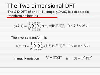
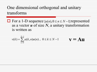
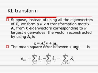
30. The Haar transform
The Haar functions hk(x) are defined on a continuous
interval, x [0,1], and for k = 0,…,N-1, where N = 2n.
The integer k can be uniquely decomposed as k = 2p + q -1
where 0 ≤ p ≤ n-1; q=0,1 for p=0 and 1 ≤ q ≤ 2p for p≠0. For
example, when, N=4
k 0 1 2 3
p 0 0 1 1
q 0 1 1 2

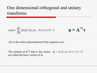
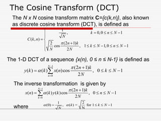
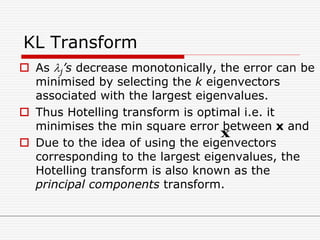
31. The Haar transform
•The Haar functions are defined as
0 0,0
/ 2
/ 2
,
1
( ) ( ) , [0,1]
1
1 22 ,
2 2
1
1 2( ) 2 ,
2 2
0, [0,1]
p
p p
p
k p q p p
h x h x x
N
q
q
x
q
q
h x h x
N
otherwise for x
  

 
 



    







32. Haar transform example
The Haar transform is obtained by letting x take discrete
values at m/ N, m=0,…,N-1. For N = 4, the transform is
1 1 1 1
1 1 1 11
2 2 0 04
0 0 2 2
 
   
 
 
  
Hr

33. Properties of Haar transform
 The Haar transform is real and
orthogonal
Hr = Hr* and Hr-1 = HrT
 Haar transform is very fast: O(N)
 The basis vectors are sequency
ordered.
 It has poor energy compaction for
images.

34. KL transform
Hotelling transform
 Originally introduced as a series
expansion for continuous random
process by Karhunen and Loeve.
 The discrete equivalent of KL series
expansion – studied by Hotelling.
 KL transform is also called the
Hotelling transform or the method of
principal components.

35. KL transform
 Let x = {x1, x2,…, xn}T be the n x 1 random
vector.
 For K vector samples from a random
population, the mean vector is given by
 The covariance matrix of the population is
given by
1
1 K
k
kK 
 xm x
1
1 K
T T
k k
kK 
 x x xC x x m m

36. KL Transform
 Cx is n x n real and symmetric matrix.
 Therefore a set on n orthonormal eigenvectors
is possible.
 Let ei and i, i=1, 2, …, n, be the eigenvectors
and corresponding eigenvalues of Cx, arranged
in descending order so that j ≥ i+1 for j = 1, 2,
…, n.
 Let A be a matrix whose rows are formed from
the eigenvectors of Cx, ordered so that first row
of A is eigenvector corresponding to the largest
eigenvalue, and the last row is the eigenvector
corresponding to the smallest eigenvalue.

37. KL Transform
 Suppose we use A as a transformation
matrix to map the vectors x’s into the
vectors y’s as follows:
y = A(x – mx)
This expression is called the Hotelling
transform.
 The mean of the y vectors resulting from
this transformation is zero; that is my =
E{y} =0.

38. KL Transform
 The covarianve matrix of the y’s is given in
terms of A and Cx by the expression
Cy = ACxAT
 Cy is a diagonal matrix whose elements along
the main diagonal are the eigenvalues of Cx
1
2
0
0 n



 
 
 
 
 
 
yC

39. KL Transform
 The off-diagonal elements of this
covariance matrix are 0, so that the
elements of the y vectors are
uncorrelated.
 Cx and Cy have the same eigenvalues
and eigenvectors.
 The inverse transformation is given by
x = ATy + mx

40. KL transform
 Suppose, instead of using all the eigenvectors
of Cx we form a k x n transformation matrix
Ak from k eigenvectors corresponding to k
largest eigenvalues, the vector reconstructed
by using Ak is
 The mean square error between x and is
T
k xx = A y + m
x
1 1 1
n k n
ms j j j
j j j K
e   
   
    

41. KL Transform
 As j’s decrease monotonically, the error can be
minimised by selecting the k eigenvectors
associated with the largest eigenvalues.
 Thus Hotelling transform is optimal i.e. it
minimises the min square error between x and
 Due to the idea of using the eigenvectors
corresponding to the largest eigenvalues, the
Hotelling transform is also known as the
principal components transform.
x

42. KL transform example
2 3 4
0 1 1 1
0 0 1 0
0 0 0 1
       
                 
              
1x x x x
3 1 1
1
1 3 1
16
1 1 3
 
  
  
xC =
3
1
1
4
1
 
   
  
xm
0.5774 0.5774 0.5774
-0.1543 -0.7715 0.6172
0.8018 0.2673 0.5345
A
 
 
 
  
=
1 2 30.0625 0.2500 0.2500    
0.1443 -0.4330 0.1443 0.1443
0.1543 -0.0000 -0.7715 0.6172
-0.8018 0.0000 0.2673 0.5345
 
 
 
  
y =
0
0
0
 
   
  
ym
0.0833 0.0000 0.0000
0.0000 0.3333 0.0000
0.0000 0.0000 0.3333
 
 
 
  
yC =

43. a) Original Image,
b) Reconstructed using all the three principal components,
c) Reconstructed image using two largest principal components,
d) Reconstructed image using only the largest principal component
KL Transform Example
a b
c d