The document discusses linear transformations between vector spaces. It defines key concepts such as the domain, codomain, image, and preimage of a transformation. A linear transformation preserves vector addition and scalar multiplication. Any function defined by a matrix T(v) = Av is a linear transformation from Rn to Rm. The matrix representing a linear transformation describes how it rotates vectors in the plane.

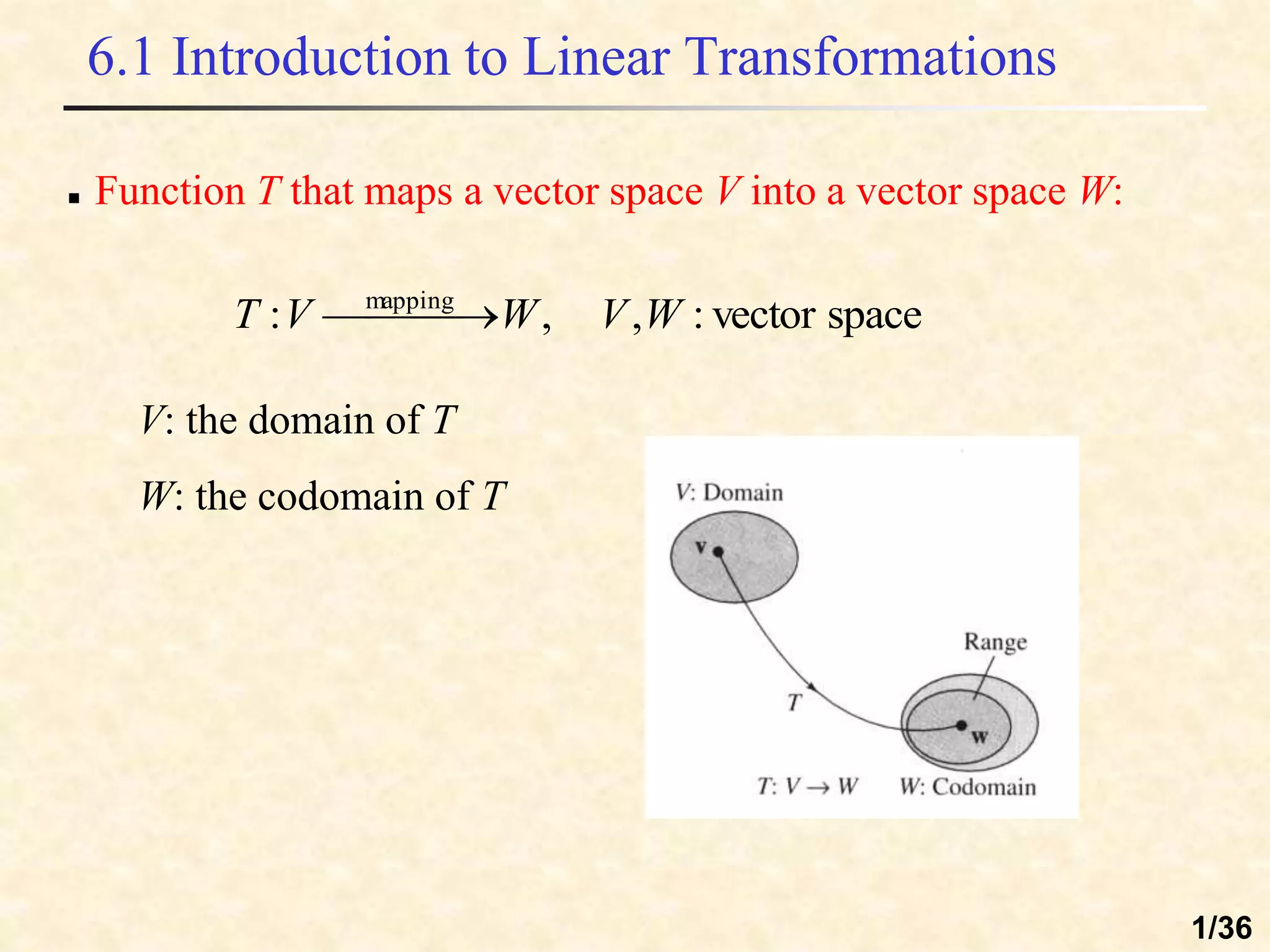
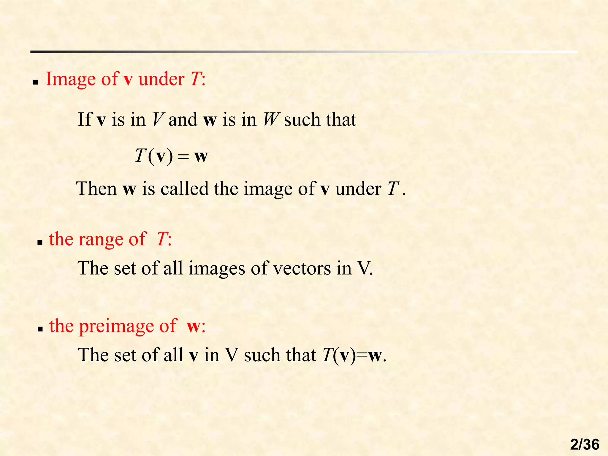
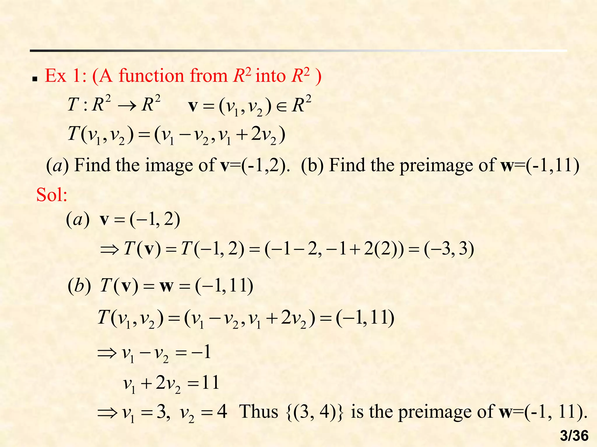
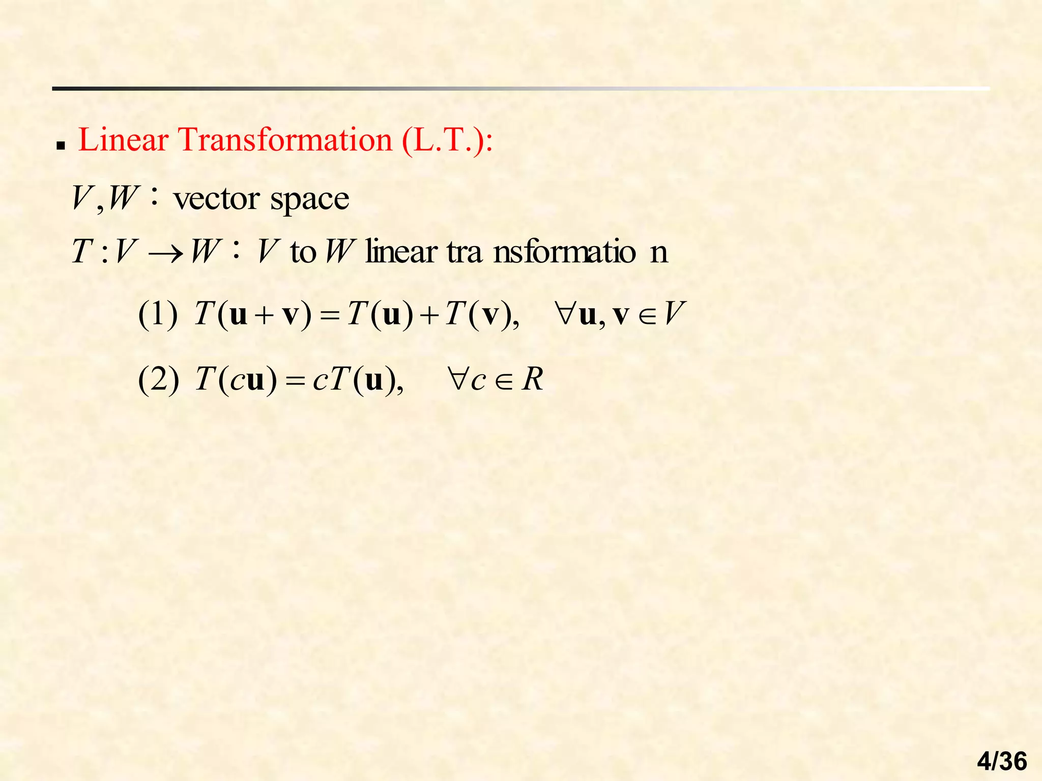
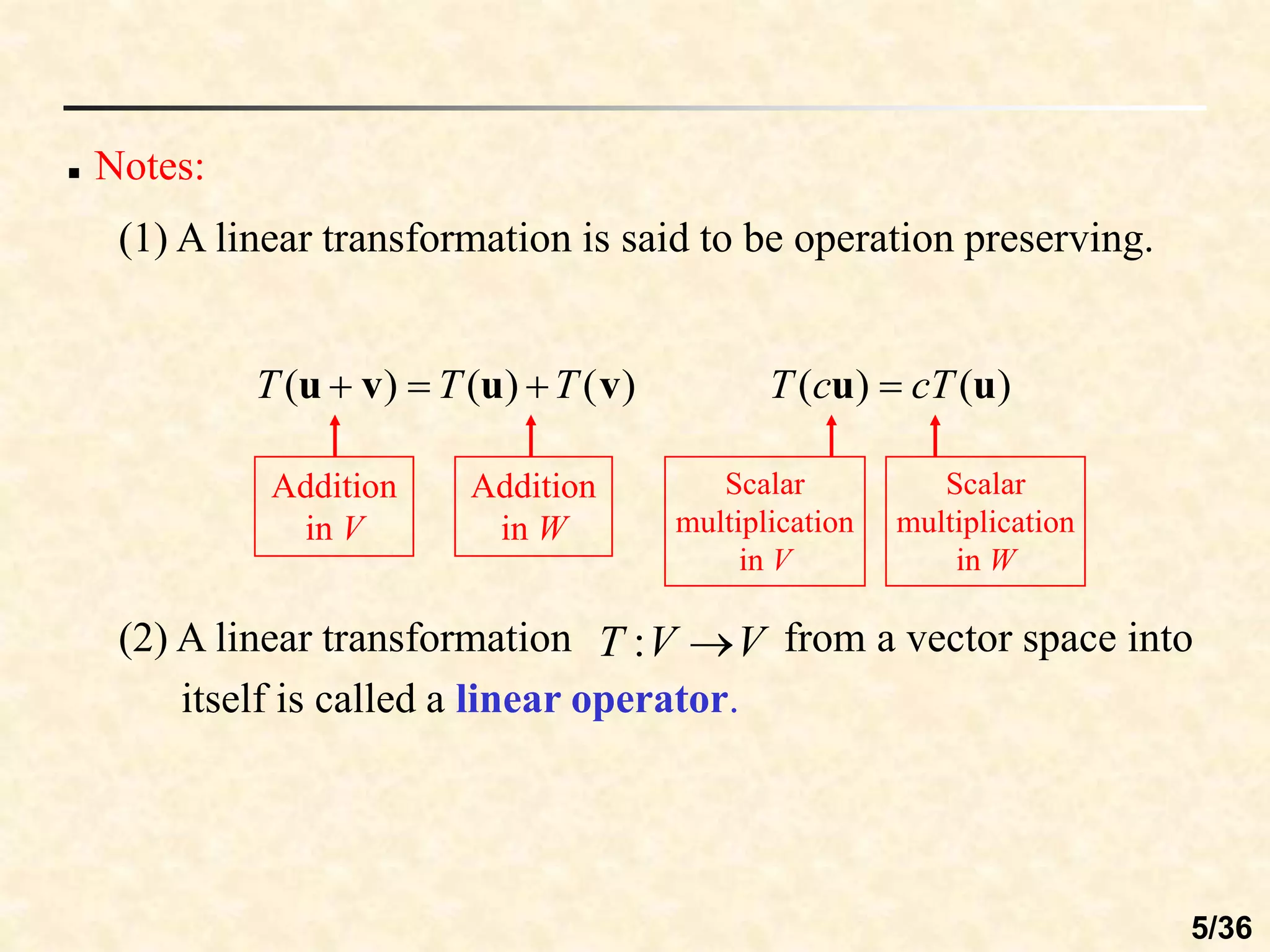
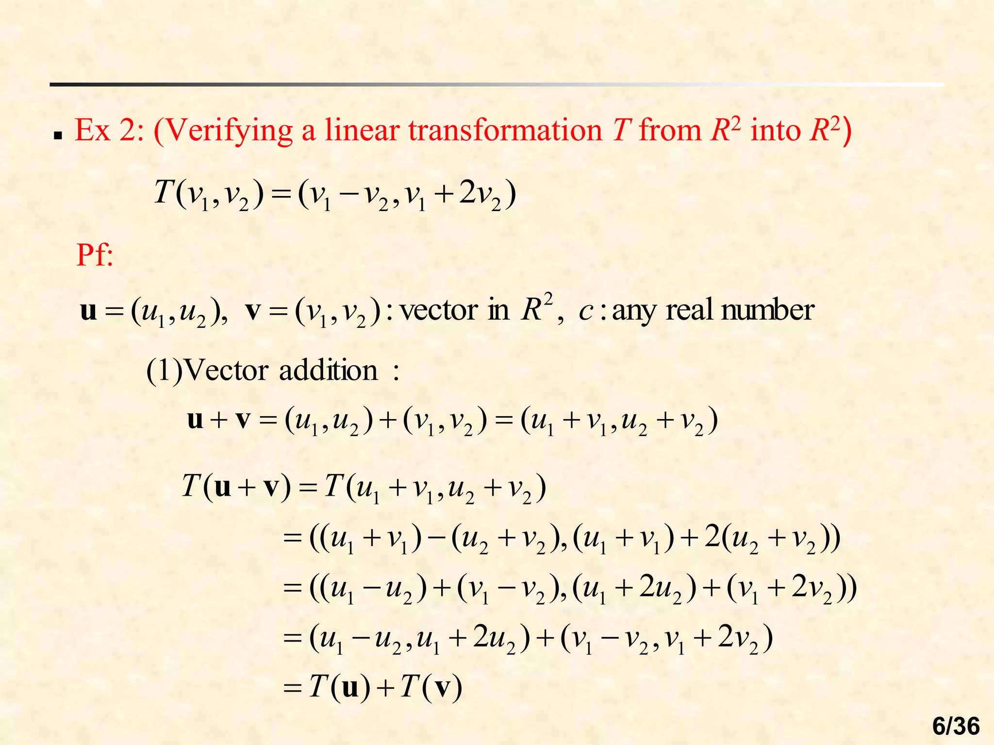
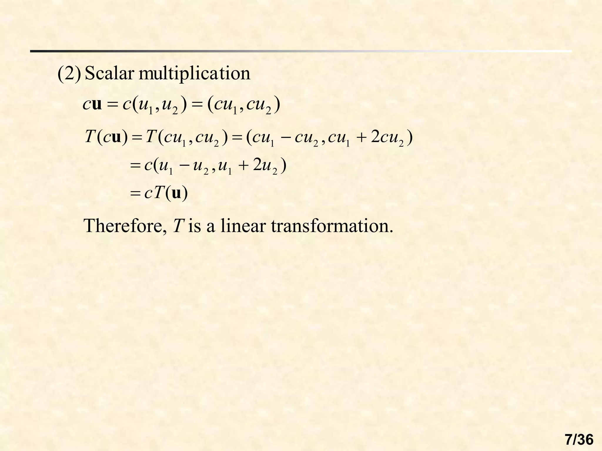
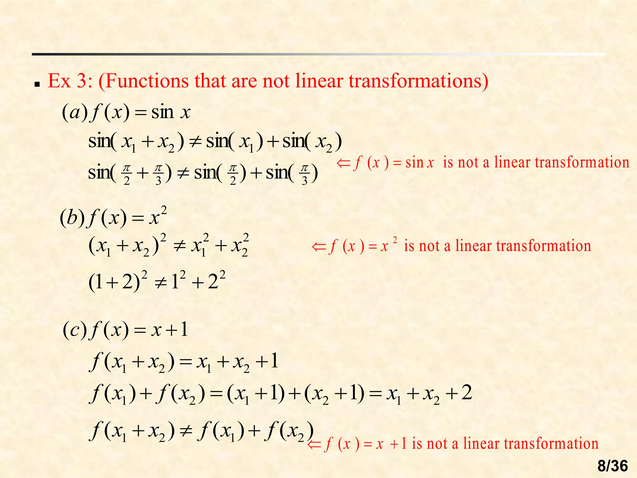
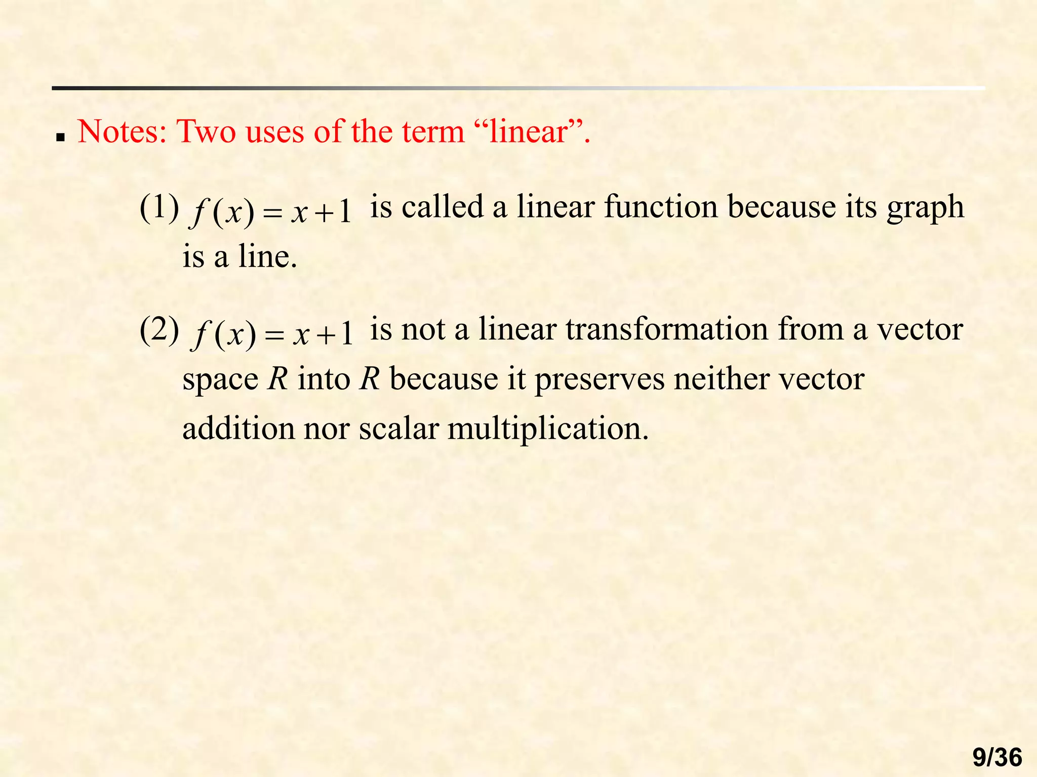
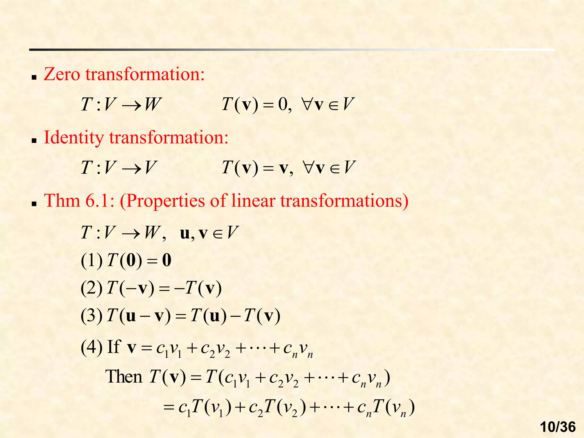
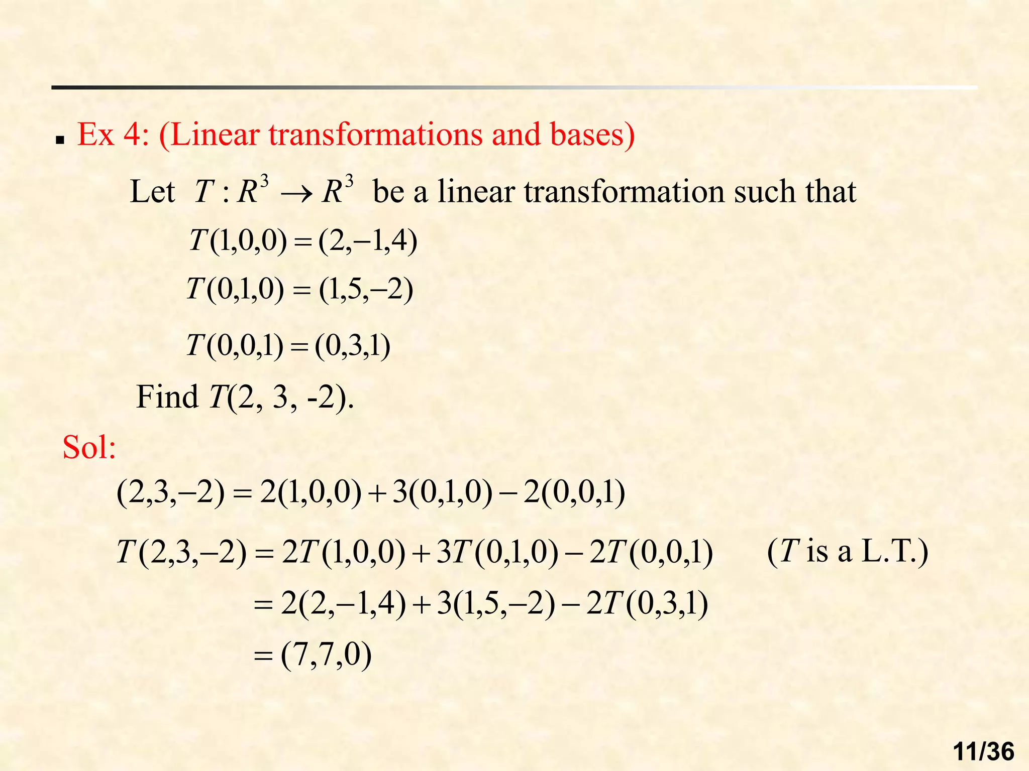
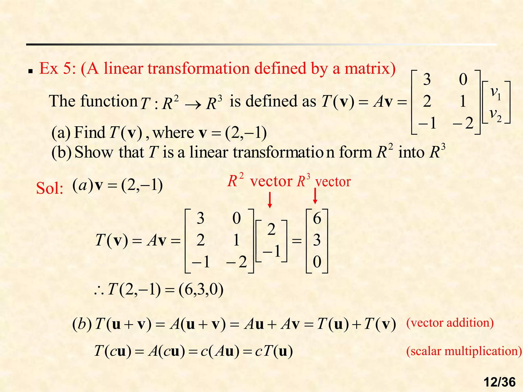
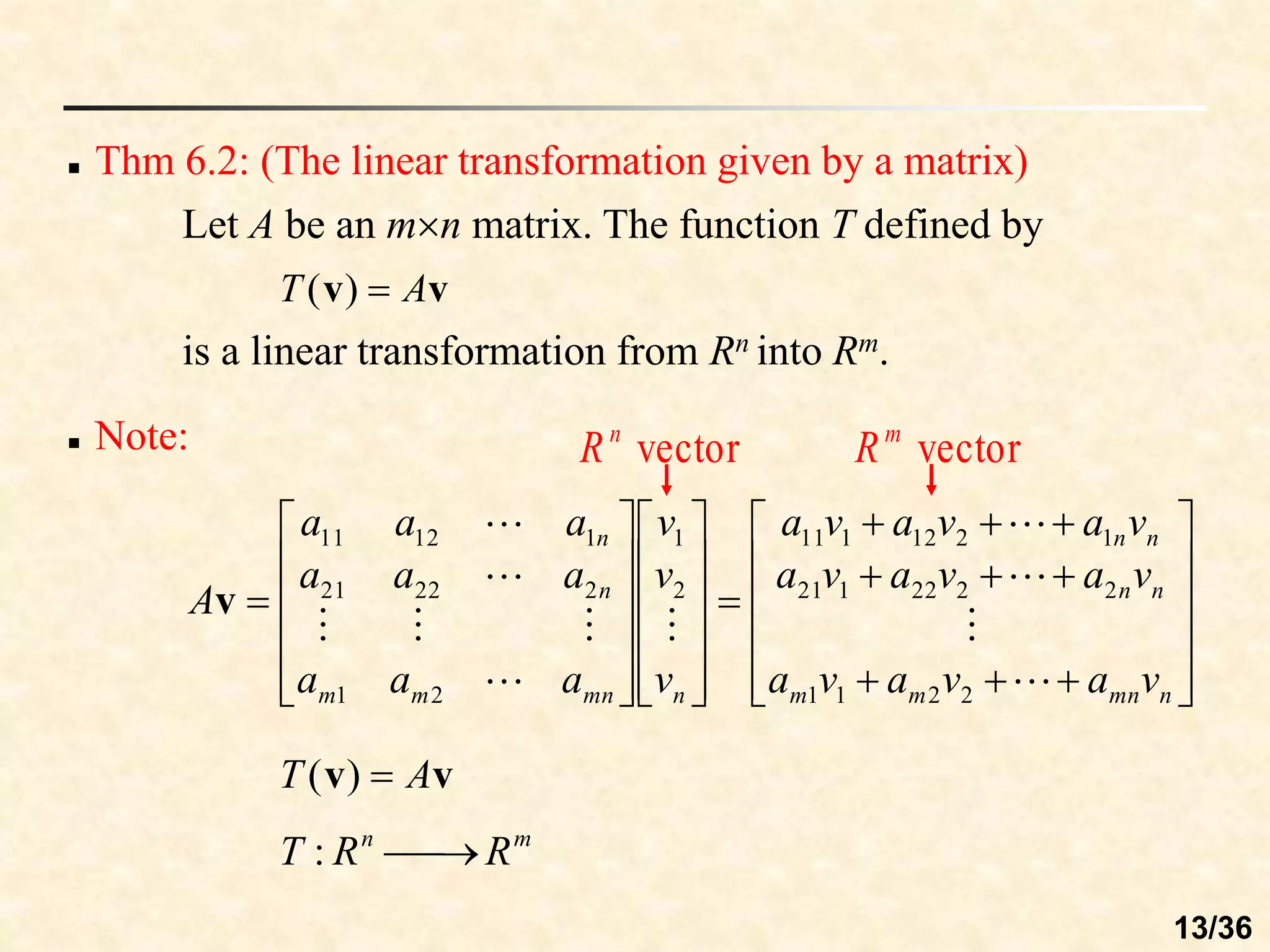
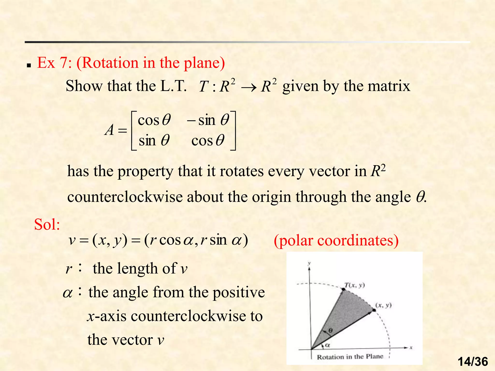
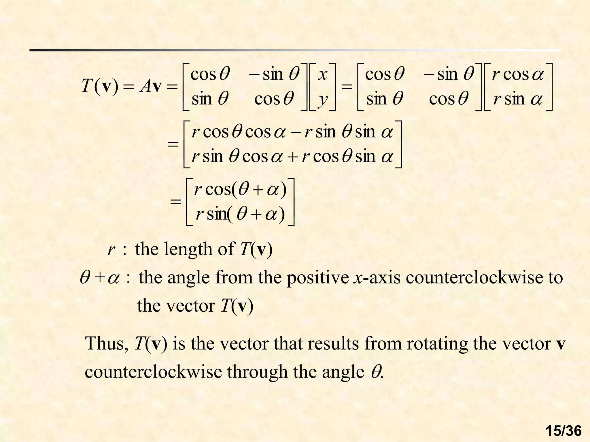
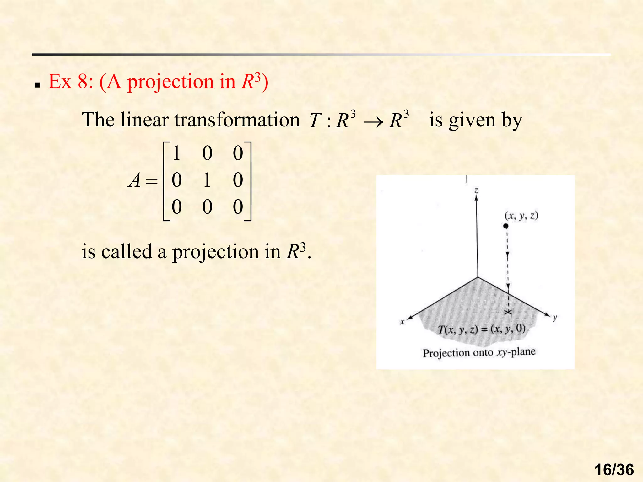
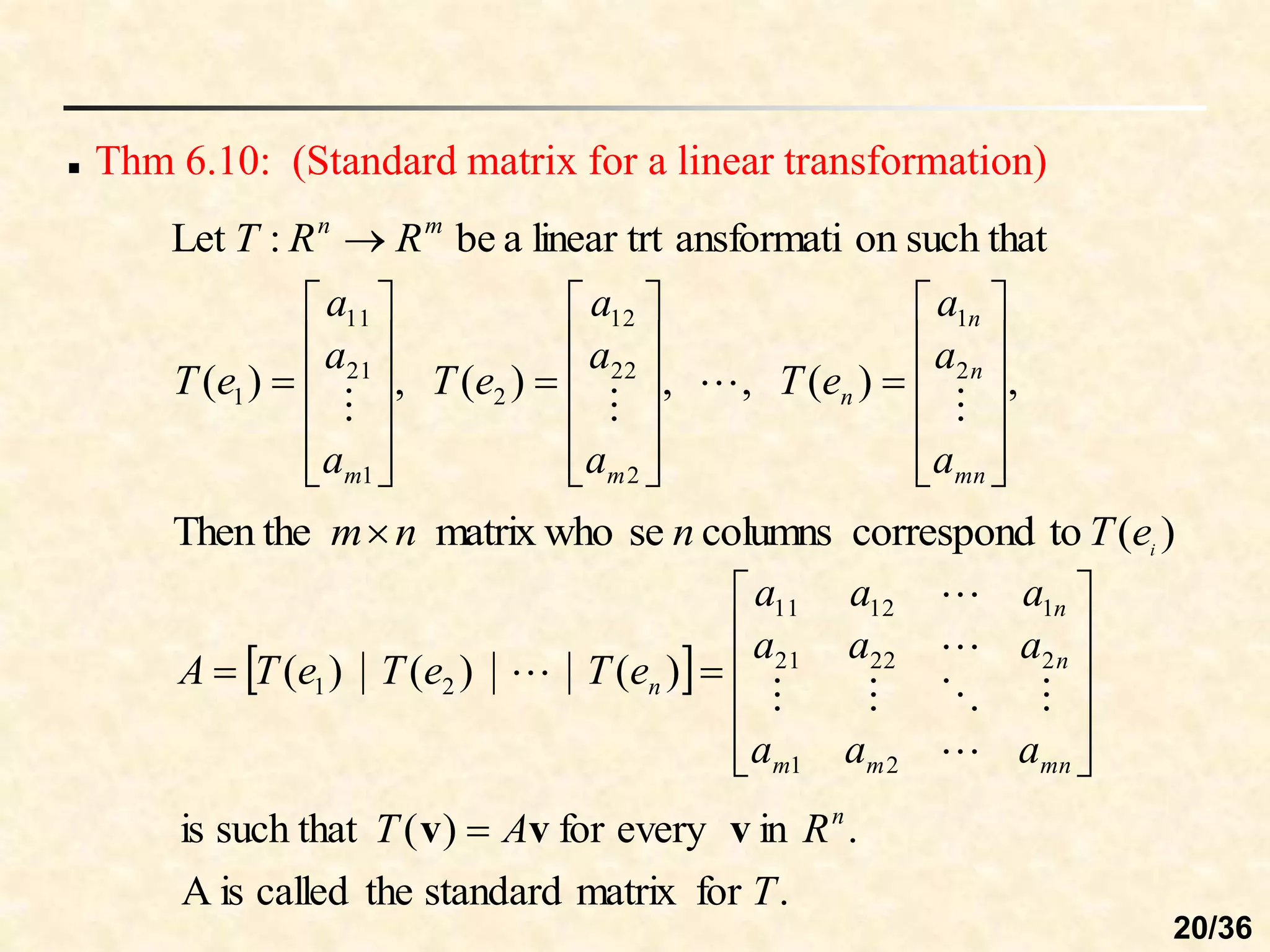
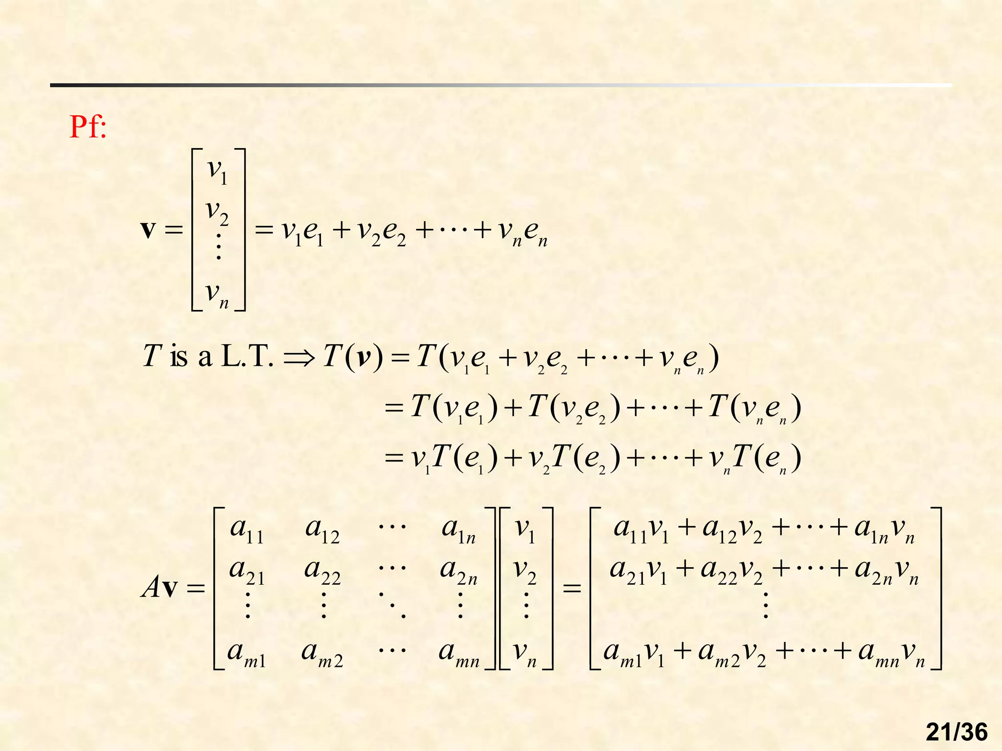
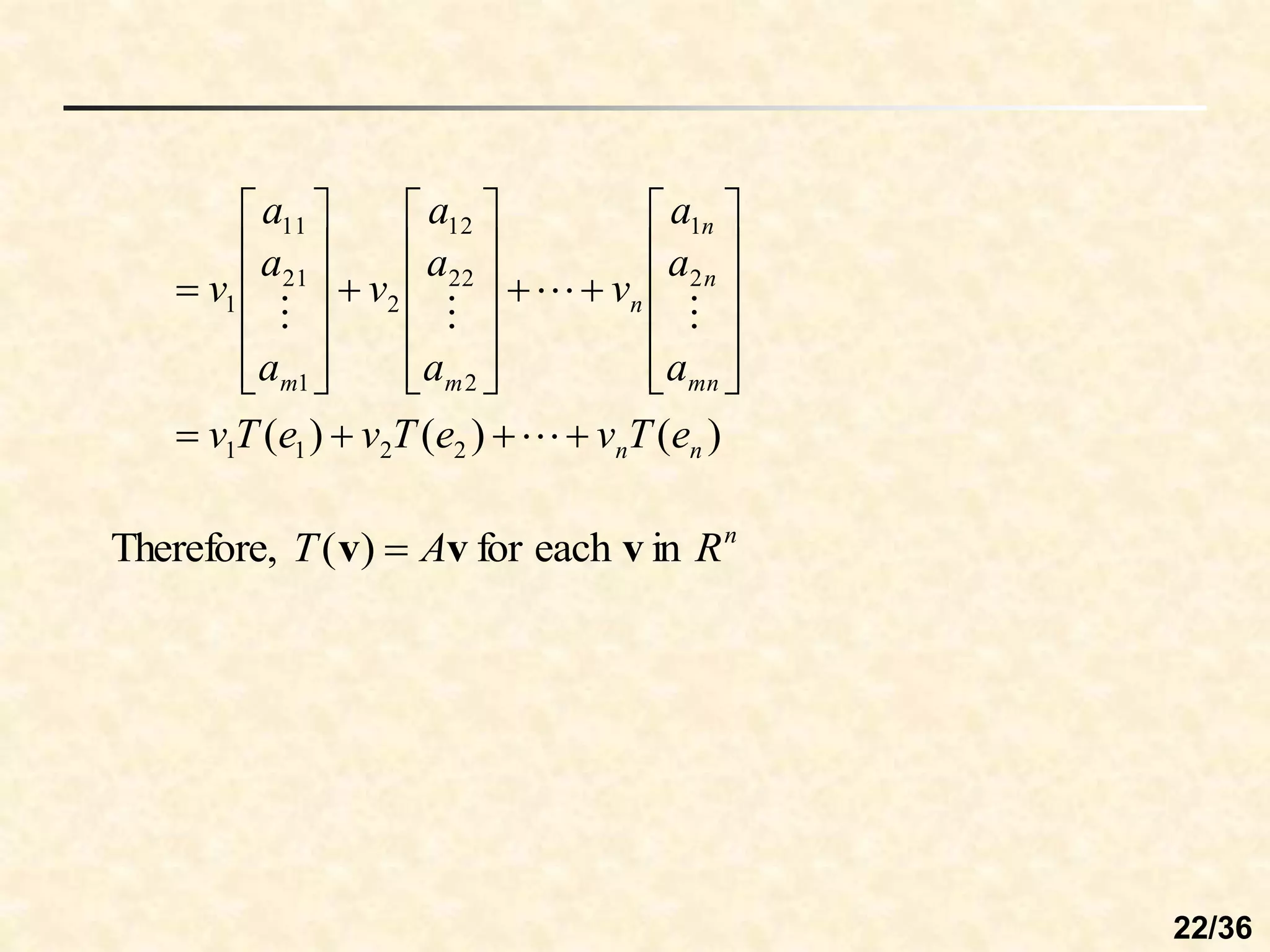
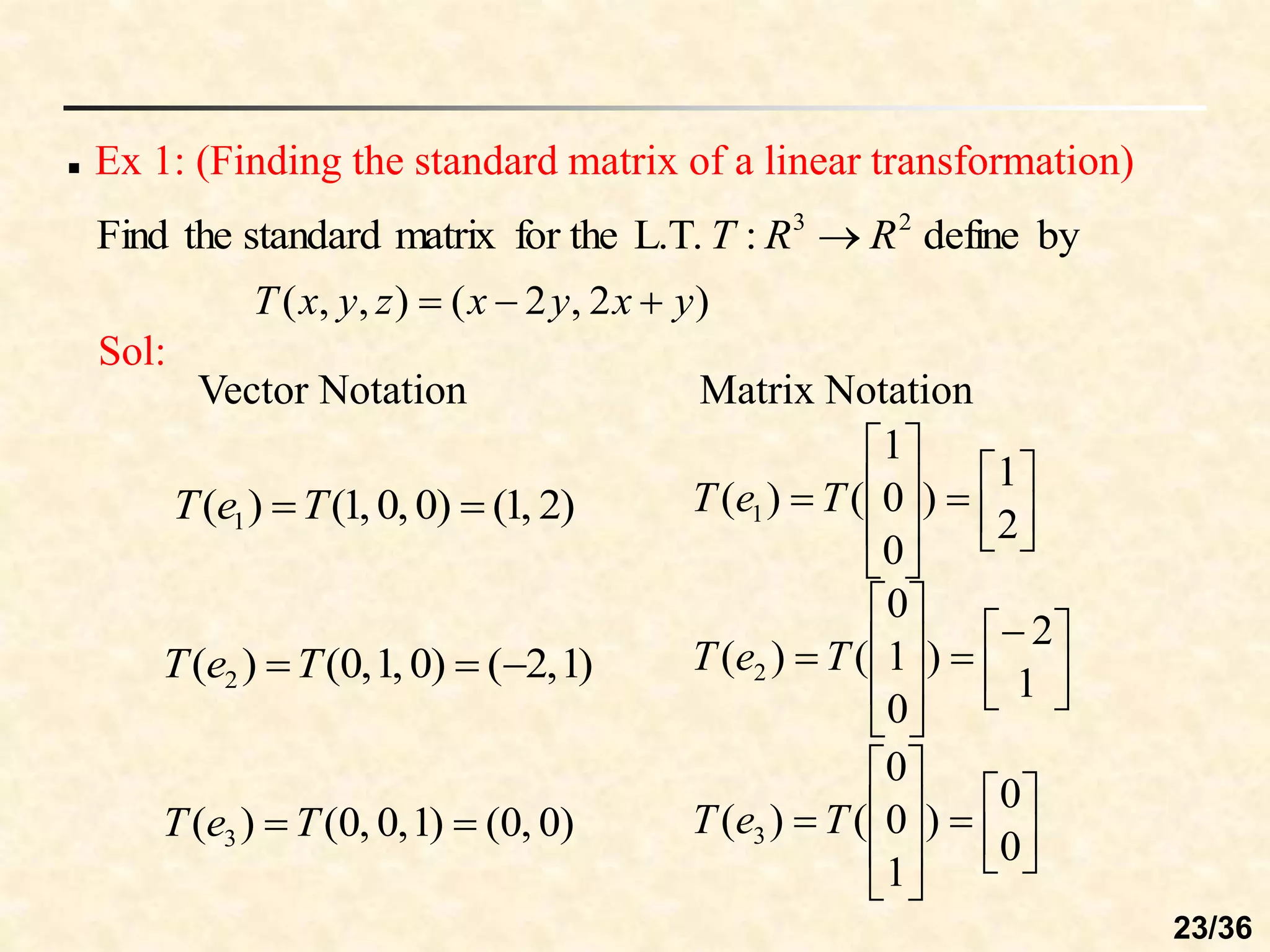
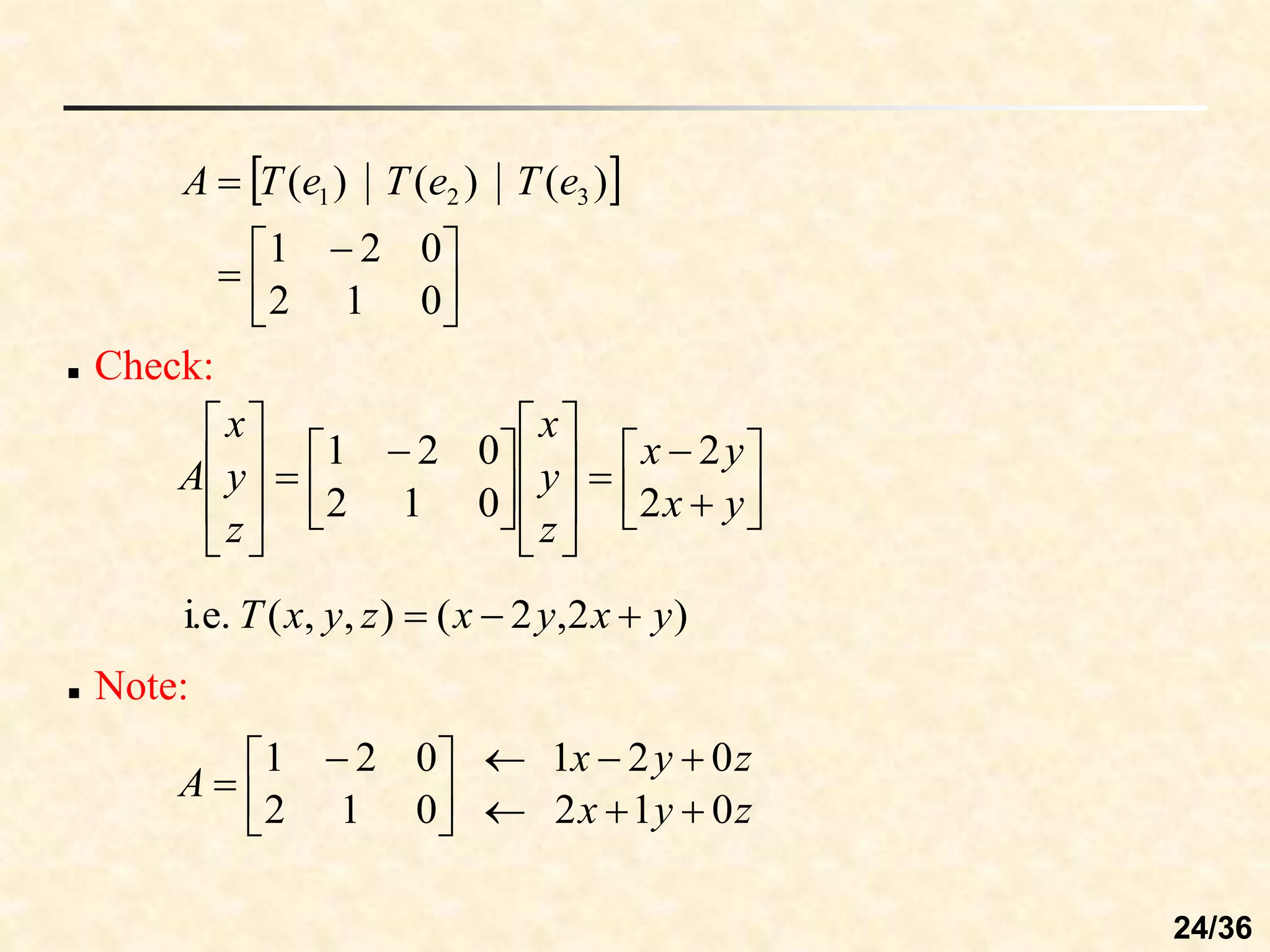
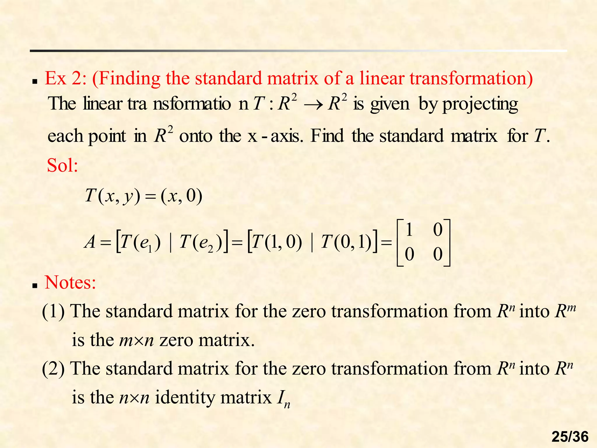
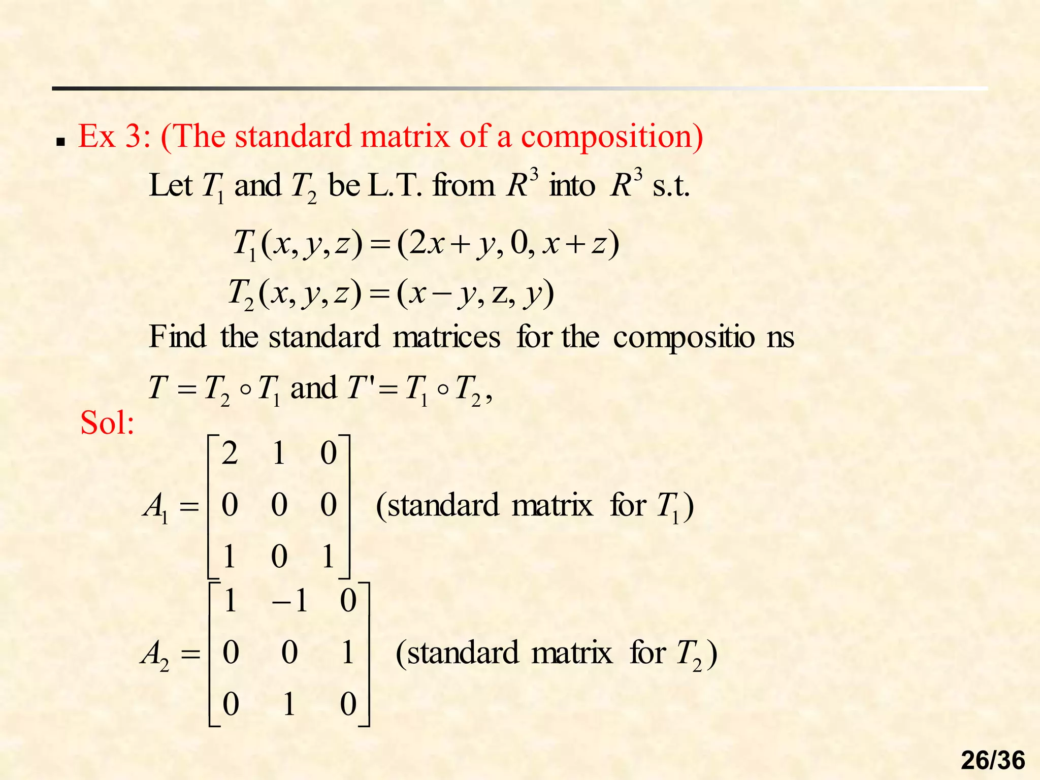
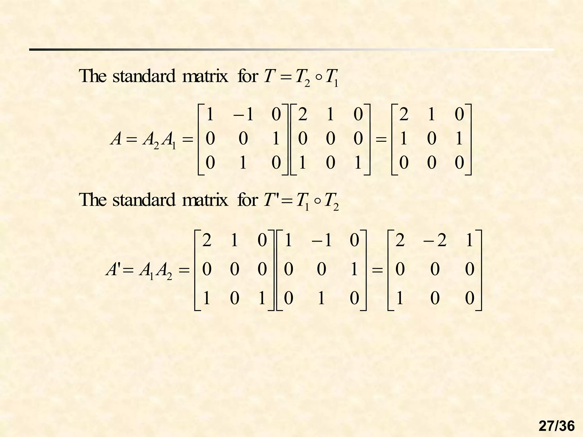
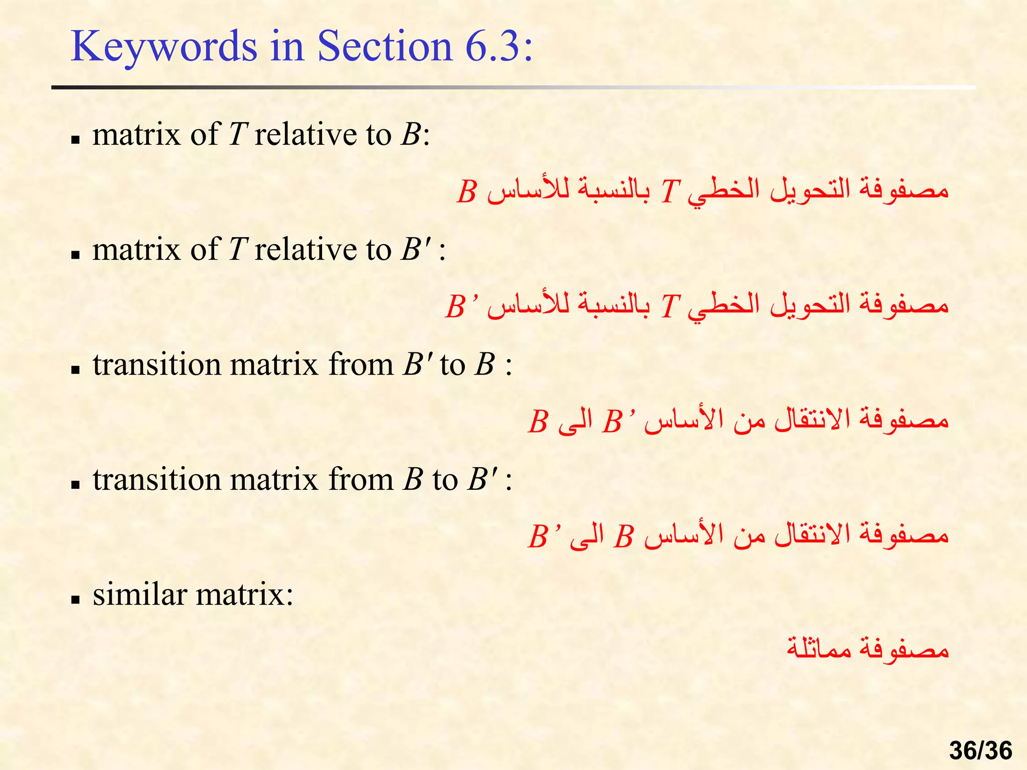
1. Chapter 6
Linear Transformations
6.1 Introduction to Linear Transformations
6.2 Matrices for Linear Transformations
6.3 Similarity

2. 6.1 Introduction to Linear Transformations
 Function T that maps a vector space V into a vector space W:
space
vector
:
,
,
: mapping
W
V
W
V
T 

 

V: the domain of T
W: the codomain of T
1/36

3.  Image of v under T:
If v is in V and w is in W such that
w
v 
)
(
T
Then w is called the image of v under T .
 the range of T:
The set of all images of vectors in V.
 the preimage of w:
The set of all v in V such that T(v)=w.
2/36

4.  Ex 1: (A function from R2 into R2 )
2
2
: R
R
T 
)
2
,
(
)
,
( 2
1
2
1
2
1 v
v
v
v
v
v
T 


2
2
1 )
,
( R
v
v 

v
(a) Find the image of v=(-1,2). (b) Find the preimage of w=(-1,11)
Sol:
)
3
,
3
(
))
2
(
2
1
,
2
1
(
)
2
,
1
(
)
(
)
2
,
1
(
)
(












T
T
a
v
v
)
11
,
1
(
)
(
)
( 

 w
v
T
b
)
11
,
1
(
)
2
,
(
)
,
( 2
1
2
1
2
1 



 v
v
v
v
v
v
T
11
2
1
2
1
2
1






v
v
v
v
4
,
3 2
1 

 v
v Thus {(3, 4)} is the preimage of w=(-1, 11).
3/36

5.  Linear Transformation (L.T.):
n
nsformatio
linear tra
to
：
:
space
vector
：
,
W
V
W
V
T
W
V

V
T
T
T 



 v
u
v
u
v
u ,
),
(
)
(
)
(
(1)
R
c
cT
c
T 

 ),
(
)
(
)
2
( u
u
4/36

6.  Notes:
(1) A linear transformation is said to be operation preserving.
)
(
)
(
)
( v
u
v
u T
T
T 


Addition
in V
Addition
in W
)
(
)
( u
u cT
c
T 
Scalar
multiplication
in V
Scalar
multiplication
in W
(2) A linear transformation from a vector space into
itself is called a linear operator.
V
V
T 
:
5/36

7.  Ex 2: (Verifying a linear transformation T from R2 into R2)
Pf:
)
2
,
(
)
,
( 2
1
2
1
2
1 v
v
v
v
v
v
T 


number
real
any
:
,
in
vector
:
)
,
(
),
,
( 2
2
1
2
1 c
R
v
v
u
u 
 v
u
)
,
(
)
,
(
)
,
(
:
addition
(1)Vector
2
2
1
1
2
1
2
1 v
u
v
u
v
v
u
u 




 v
u
)
(
)
(
)
2
,
(
)
2
,
(
))
2
(
)
2
(
),
(
)
((
))
(
2
)
(
),
(
)
((
)
,
(
)
(
2
1
2
1
2
1
2
1
2
1
2
1
2
1
2
1
2
2
1
1
2
2
1
1
2
2
1
1
v
u
v
u
T
T
v
v
v
v
u
u
u
u
v
v
u
u
v
v
u
u
v
u
v
u
v
u
v
u
v
u
v
u
T
T


























6/36

8. )
,
(
)
,
(
tion
multiplica
Scalar
)
2
(
2
1
2
1 cu
cu
u
u
c
c 

u
)
(
)
2
,
(
)
2
,
(
)
,
(
)
(
2
1
2
1
2
1
2
1
2
1
u
u
cT
u
u
u
u
c
cu
cu
cu
cu
cu
cu
T
c
T








Therefore, T is a linear transformation.
7/36

9.  Ex 3: (Functions that are not linear transformations)
x
x
f
a sin
)
(
)
( 
2
)
(
)
( x
x
f
b 
1
)
(
)
( 
 x
x
f
c
)
sin(
)
sin(
)
sin( 2
1
2
1 x
x
x
x 


)
sin(
)
sin(
)
sin( 3
2
3
2







2
2
2
1
2
2
1 )
( x
x
x
x 


2
2
2
2
1
)
2
1
( 


1
)
( 2
1
2
1 


 x
x
x
x
f
2
)
1
(
)
1
(
)
(
)
( 2
1
2
1
2
1 






 x
x
x
x
x
f
x
f
)
(
)
(
)
( 2
1
2
1 x
f
x
f
x
x
f 


( ) sin is not a linear transformation
f x x
 
2
( ) is not a linear transformation
f x x
 
( ) 1 is not a linear transformation
f x x
  
8/36

10.  Notes: Two uses of the term “linear”.
(1) is called a linear function because its graph
is a line.
1
)
( 
 x
x
f
(2) is not a linear transformation from a vector
space R into R because it preserves neither vector
addition nor scalar multiplication.
1
)
( 
 x
x
f
9/36

11.  Zero transformation:
V
W
V
T 
 v
u,
,
:
V
T 

 v
v ,
0
)
(
 Identity transformation:
V
V
T 
: V
T 

 v
v
v ,
)
(
 Thm 6.1: (Properties of linear transformations)
W
V
T 
:
0
0 
)
(
(1) T
)
(
)
(
(2) v
v T
T 


)
(
)
(
)
(
(3) v
u
v
u T
T
T 


)
(
)
(
)
(
)
(
)
(
Then
If
(4)
2
2
1
1
2
2
1
1
2
2
1
1
n
n
n
n
n
n
v
T
c
v
T
c
v
T
c
v
c
v
c
v
c
T
T
v
c
v
c
v
c















v
v
10/36

12.  Ex 4: (Linear transformations and bases)
Let be a linear transformation such that
3
3
: R
R
T 
)
4
,
1
,
2
(
)
0
,
0
,
1
( 

T
)
2
,
5
,
1
(
)
0
,
1
,
0
( 

T
)
1
,
3
,
0
(
)
1
,
0
,
0
( 
T
Sol:
)
1
,
0
,
0
(
2
)
0
,
1
,
0
(
3
)
0
,
0
,
1
(
2
)
2
,
3
,
2
( 



)
0
,
7
,
7
(
)
1
,
3
,
0
(
2
)
2
,
5
,
1
(
3
)
4
,
1
,
2
(
2
)
1
,
0
,
0
(
2
)
0
,
1
,
0
(
3
)
0
,
0
,
1
(
2
)
2
,
3
,
2
(










T
T
T
T
T (T is a L.T.)
Find T(2, 3, -2).
11/36

13.  Ex 5: (A linear transformation defined by a matrix)
The function is defined as
3
2
: R
R
T  

















2
1
2
1
1
2
0
3
)
(
v
v
A
T v
v
3
2
into
form
n
nsformatio
linear tra
a
is
that
Show
(b)
)
1
,
2
(
where
,
)
(
Find
(a)
R
R
T
T 

v
v
Sol: )
1
,
2
(
)
( 

v
a




























0
3
6
1
2
2
1
1
2
0
3
)
( v
v A
T
)
0
,
3
,
6
(
)
1
,
2
( 

T
vector
2
R vector
3
R
)
(
)
(
)
(
)
(
)
( v
u
v
u
v
u
v
u T
T
A
A
A
T
b 






)
(
)
(
)
(
)
( u
u
u
u cT
A
c
c
A
c
T 


(vector addition)
(scalar multiplication)
12/36

14.  Thm 6.2: (The linear transformation given by a matrix)
Let A be an mn matrix. The function T defined by
v
v A
T 
)
(
is a linear transformation from Rn into Rm.
 Note:















































n
mn
m
m
n
n
n
n
n
mn
m
m
n
n
v
a
v
a
v
a
v
a
v
a
v
a
v
a
v
a
v
a
v
v
v
a
a
a
a
a
a
a
a
a
A











2
2
1
1
2
2
22
1
21
1
2
12
1
11
2
1
2
1
2
22
21
1
12
11
v
v
v A
T 
)
(
m
n
R
R
T 

:
vector
n
R vector
m
R
13/36

15. Show that the L.T. given by the matrix
has the property that it rotates every vector in R2
counterclockwise about the origin through the angle .
 Ex 7: (Rotation in the plane)
2
2
: R
R
T 





 





cos
sin
sin
cos
A
Sol:
)
sin
,
cos
(
)
,
( 
 r
r
y
x
v 
 (polar coordinates)
r： the length of v
：the angle from the positive
x-axis counterclockwise to
the vector v
14/36

16. 




























 












 


)
sin(
)
cos(
sin
cos
cos
sin
sin
sin
cos
cos
sin
cos
cos
sin
sin
cos
cos
sin
sin
cos
)
(






















r
r
r
r
r
r
r
r
y
x
A
T v
v
r：the length of T(v)
 +：the angle from the positive x-axis counterclockwise to
the vector T(v)
Thus, T(v) is the vector that results from rotating the vector v
counterclockwise through the angle .
15/36

17. is called a projection in R3.
 Ex 8: (A projection in R3)
The linear transformation is given by
3
3
: R
R
T 









0
0
0
0
1
0
0
0
1
A
16/36

18. Show that T is a linear transformation.
 Ex 9: (A linear transformation from Mmn into Mn m )
)
:
(
)
( m
n
n
m
T
M
M
T
A
A
T 
 

Sol:
n
m
M
B
A 

,
)
(
)
(
)
(
)
( B
T
A
T
B
A
B
A
B
A
T T
T
T







)
(
)
(
)
( A
cT
cA
cA
cA
T T
T



Therefore, T is a linear transformation from Mmn into Mn m.
17/36

19. Keywords in Section 6.1:
 function: ‫دالة‬
 domain: ‫مجال‬
 codomain: ‫مقابل‬ ‫مجال‬
 image of v under T: ‫التحويل‬ ‫تحت‬ ‫صورة‬
 range of T: T ‫مدى‬
 preimage of w:
 linear transformation: ‫خطي‬ ‫تحويل‬
 linear operator: ‫خطي‬ ‫مؤثر‬
 zero transformation: ‫صفري‬ ‫تحويل‬
 identity transformation: ‫محايد‬ ‫تحويل‬
v
T
18/36

20. 6.2 Matrices for Linear Transformations
)
4
3
,
2
3
,
2
(
)
,
,
(
)
1
( 3
2
3
2
1
3
2
1
3
2
1 x
x
x
x
x
x
x
x
x
x
x
T 






 Three reasons for matrix representation of a linear transformation:





















3
2
1
4
3
0
2
3
1
1
1
2
)
(
)
2
(
x
x
x
A
T x
x
 It is simpler to write.
 It is simpler to read.
 It is more easily adapted for computer use.
 Two representations of the linear transformation T:R3→R3 :
19/36

21.  Thm 6.10: (Standard matrix for a linear transformation)
such that
on
ansformati
linear trt
a
be
:
Let m
n
R
R
T 
,
)
(
,
,
)
(
,
)
( 2
1
2
22
12
2
1
21
11
1







































mn
n
n
n
m
m a
a
a
e
T
a
a
a
e
T
a
a
a
e
T




)
(
to
correspond
columns
se
matrix who
Then the i
e
T
n
n
m
.
for
matrix
standard
the
called
is
A
.
in
every
for
)
(
such that
is
T
R
A
T n
v
v
v 
 














mn
m
m
n
n
n
a
a
a
a
a
a
a
a
a
e
T
e
T
e
T
A








2
1
2
22
21
1
12
11
2
1 )
(
)
(
)
(
20/36

22. Pf:
n
n
n
e
v
e
v
e
v
v
v
v
















 
 2
2
1
1
2
1
v
)
(
)
(
)
(
)
(
)
(
)
(
)
(
)
(
L.T.
a
is
2
2
1
1
2
2
1
1
2
2
1
1
n
n
n
n
n
n
e
T
v
e
T
v
e
T
v
e
v
T
e
v
T
e
v
T
e
v
e
v
e
v
T
T
T
















v















































n
mn
m
m
n
n
n
n
n
mn
m
m
n
n
v
a
v
a
v
a
v
a
v
a
v
a
v
a
v
a
v
a
v
v
v
a
a
a
a
a
a
a
a
a
A












2
2
1
1
2
2
22
1
21
1
2
12
1
11
2
1
2
1
2
22
21
1
12
11
v
21/36

23. )
(
)
(
)
( 2
2
1
1
2
1
2
22
12
2
1
21
11
1
n
n
mn
n
n
n
m
m
e
T
v
e
T
v
e
T
v
a
a
a
v
a
a
a
v
a
a
a
v

















































n
R
A
T in
each
for
)
(
Therefore, v
v
v 
22/36

24.  Ex 1: (Finding the standard matrix of a linear transformation)
by
define
:
L.T.
for the
matrix
standard
the
Find 2
3
R
R
T 
)
2
,
2
(
)
,
,
( y
x
y
x
z
y
x
T 


Sol:
)
2
,
1
(
)
0
,
0
,
1
(
)
( 1 
T
e
T
)
1
,
2
(
)
0
,
1
,
0
(
)
( 2 

T
e
T
)
0
,
0
(
)
1
,
0
,
0
(
)
( 3 
 T
e
T
2
1
)
0
0
1
(
)
( 1 














 T
e
T
1
2
)
0
1
0
(
)
( 2 














 T
e
T
0
0
)
1
0
0
(
)
( 3 














 T
e
T
Vector Notation Matrix Notation
23/36

25.  





 


0
1
2
0
2
1
)
(
)
(
)
( 3
2
1 e
T
e
T
e
T
A
 Note:
z
y
x
z
y
x
A
0
1
2
0
2
1
0
1
2
0
2
1











 























 









y
x
y
x
z
y
x
z
y
x
A
2
2
0
1
2
0
2
1
)
2
,
2
(
)
,
,
(
i.e. y
x
y
x
z
y
x
T 


 Check:
24/36

26.  Ex 2: (Finding the standard matrix of a linear transformation)
.
for
matrix
standard
the
Find
axis.
-
x
the
onto
in
point
each
projecting
by
given
is
:
n
nsformatio
linear tra
The
2
2
2
T
R
R
R
T 
Sol:
)
0
,
(
)
,
( x
y
x
T 
    








0
0
0
1
)
1
,
0
(
)
0
,
1
(
)
(
)
( 2
1 T
T
e
T
e
T
A
 Notes:
(1) The standard matrix for the zero transformation from Rn into Rm
is the mn zero matrix.
(2) The standard matrix for the zero transformation from Rn into Rn
is the nn identity matrix In
25/36

27.  Ex 3: (The standard matrix of a composition)
s.t.
into
from
L.T.
be
and
Let 3
3
2
1 R
R
T
T
)
,
0
,
2
(
)
,
,
(
1 z
x
y
x
z
y
x
T 


)
,
z
,
(
)
,
,
(
2 y
y
x
z
y
x
T 

,
'
and
ns
compositio
for the
matrices
standard
the
Find
2
1
1
2 T
T
T
T
T
T 
 

Sol:
)
for
matrix
standard
(
1
0
1
0
0
0
0
1
2
1
1 T
A











)
for
matrix
standard
(
0
1
0
1
0
0
0
1
1
2
2 T
A









 

26/36

28. 1
2
for
matrix
standard
The T
T
T 

2
1
'
for
matrix
standard
The T
T
T 

























 


0
0
0
1
0
1
0
1
2
1
0
1
0
0
0
0
1
2
0
1
0
1
0
0
0
1
1
1
2 A
A
A









 










 












0
0
1
0
0
0
1
2
2
0
1
0
1
0
0
0
1
1
1
0
1
0
0
0
0
1
2
' 2
1A
A
A
27/36

29.  Inverse linear transformation:
in
every
for
s.t.
L.T.
are
:
and
:
If 2
1
n
n
n
n
n
R
R
R
T
R
R
T v


))
(
(
and
))
(
( 2
1
1
2 v
v
v
v 
 T
T
T
T
invertible
be
to
said
is
and
of
inverse
the
called
is
Then 1
1
2 T
T
T
 Note:
If the transformation T is invertible, then the inverse is
unique and denoted by T–1 .
28/36

30.  Ex 5: (Finding a matrix relative to nonstandard bases)
by
defined
L.T.
a
be
：
Let 2
2
R
R
T 
)
2
,
(
)
,
( 2
1
2
1
2
1 x
x
x
x
x
x
T 


)}
1
,
0
(
),
0
,
1
{(
'
and
)}
1
,
1
(
),
2
,
1
{(
basis
the
to
relative
of
matrix
the
Find


 B
B
T
Sol:
)
1
,
0
(
3
)
0
,
1
(
0
)
3
,
0
(
)
1
,
1
(
)
1
,
0
(
0
)
0
,
1
(
3
)
0
,
3
(
)
2
,
1
(








T
T
    















3
0
)
1
,
1
(
,
0
3
)
2
,
1
( '
' B
B T
T
'
and
to
relative
for
matrix
the B
B
T
   
  








3
0
0
3
)
2
,
1
(
)
2
,
1
( '
' B
B T
T
A
29/36

31.  Ex 6:
)
1
,
2
(
where
),
(
find
to
matrix
the
use
5,
Example
in
given
：
L.T.
For the 2
2


v
v
T
A
R
R
T
Sol:
)
1
,
1
(
1
)
2
,
1
(
1
)
1
,
2
( 



v
  








1
1
B
v
    























3
3
1
1
3
0
0
3
)
( ' B
B A
T v
v
)
3
,
3
(
)
1
,
0
(
3
)
0
,
1
(
3
)
( 


 v
T )}
1
,
0
(
),
0
,
1
{(
'
B
)}
1
,
1
(
),
2
,
1
{( 

B
)
3
,
3
(
)
1
2(2)
,
1
2
(
)
1
,
2
( 



T
 Check:
30/36

32. Keywords in Section 6.2:
 standard matrix for T: ‫الخطي‬ ‫للتحويل‬ ‫األساسية‬ ‫المصفوفة‬
 composition of linear transformations: ‫الخطية‬ ‫للتحويالت‬ ‫تركيب‬
 inverse linear transformation: ‫عكسي‬ ‫خطي‬ ‫تحويل‬
 matrix of T relative to the bases B and B‘ :
‫الخطي‬ ‫التحويل‬ ‫مصفوفة‬
T
‫لألساس‬ ‫بالنسبة‬
B
‫و‬
B’
 matrix of T relative to the basis B:
‫الخطي‬ ‫التحويل‬ ‫مصفوفة‬
T
‫لألساس‬ ‫بالنسبة‬
B
T
31/36

33. 6.3 Similarity
 Ex 4: (Similar matrices)
similar
are
2
1
2
3
'
and
3
1
2
2
)
( 
















 A
A
a







 
1
0
1
1
where
,
'
because 1
P
AP
P
A
similar
are
3
1
1
2
'
and
7
3
7
2
)
( 















 A
A
b









 
1
2
2
3
where
,
'
because 1
P
AP
P
A
32/36

34.  Ex 5: (A comparison of two matrices for a linear transformation)
basis.
standard
the
to
relative
:
for
matrix
the
is
2
0
0
0
1
3
0
3
1
Suppose 3
3
R
R
T
A 












)}
1
,
0
,
0
(
),
0
,
1
,
1
(
),
0
,
1
,
1
{(
'
basis
the
to
relative
for
matrix
the
Find


B
T
Sol:
     
 














1
0
0
0
1
1
0
1
1
)
1
,
0
,
0
(
)
0
,
1
,
1
(
)
0
,
1
,
1
(
matrix
standard
the
to
from
matrix
n
transitio
The
B
B
B
P
B'










 
1
0
0
0
0
2
1
2
1
2
1
2
1
1
P
33/36

35. 














































 
2
0
0
0
2
0
0
0
4
1
0
0
0
1
1
0
1
1
2
0
0
0
1
3
0
3
1
1
0
0
0
0
'
:
'
to
relative
of
matrix
2
1
2
1
2
1
2
1
1
AP
P
A
B
T
34/36

36.  Notes: Computational advantages of diagonal matrices:













n
d
d
d
D







0
0
0
0
0
0
2
1













k
n
k
k
k
d
d
d
D







0
0
0
0
0
0
)
1
( 2
1
D
DT

)
2
(
0
,
0
0
0
0
0
0
)
3
(
1
1
1
1 2
1















i
d
d
d
d
D
n







35/36

37. Keywords in Section 6.3:
 matrix of T relative to B:
‫الخطي‬ ‫التحويل‬ ‫مصفوفة‬
T
‫لألساس‬ ‫بالنسبة‬
B
 matrix of T relative to B' :
‫الخطي‬ ‫التحويل‬ ‫مصفوفة‬
T
‫لألساس‬ ‫بالنسبة‬
B’
 transition matrix from B' to B :
‫األساس‬ ‫من‬ ‫االنتقال‬ ‫مصفوفة‬
B’
‫الى‬
B
 transition matrix from B to B' :
‫األساس‬ ‫من‬ ‫االنتقال‬ ‫مصفوفة‬
B
‫الى‬
B’
 similar matrix:
‫مماثلة‬ ‫مصفوفة‬
36/36