This document discusses numerical integration using the trapezoidal rule. It begins by introducing the concept of numerical integration as a way to evaluate integrals numerically. It then describes the trapezoidal rule, explaining that it approximates the integral of a function between intervals by calculating the area of trapezoids under the function curve. The rule takes the average of the function values at the interval endpoints to estimate the area of each trapezoid. An example calculates the integral of e^-x^2 from 0 to 1 using the trapezoidal rule with n=10 subintervals. It finds the result to be approximately 0.7617562, demonstrating how to apply the rule.

1. Numerical Integration: Trapezoidal Rule
Dr. Varun Kumar
Dr. Varun Kumar (IIIT Surat) Unit 5 / Lecture-1 1 / 9

2. Outlines
1 Introduction to Numerical Integration
2 Trapezoidal Rule
3 Example
Dr. Varun Kumar (IIIT Surat) Unit 5 / Lecture-1 2 / 9

3. Introduction to Numerical Integration
Important points
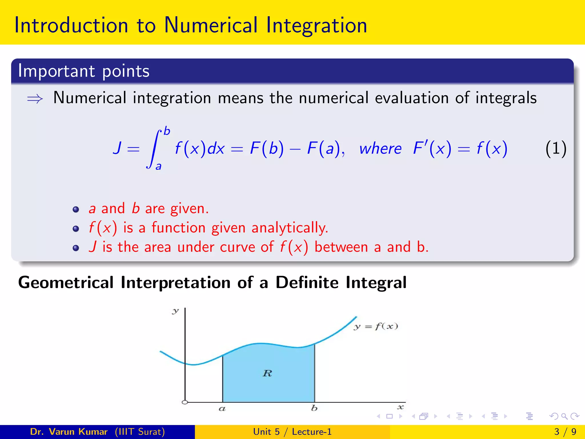
⇒ Numerical integration means the numerical evaluation of integrals
J =
Z b
a
f (x)dx = F(b) − F(a), where F0
(x) = f (x) (1)
a and b are given.
f (x) is a function given analytically.
J is the area under curve of f (x) between a and b.
Geometrical Interpretation of a Definite Integral
Dr. Varun Kumar (IIIT Surat) Unit 5 / Lecture-1 3 / 9

4. Rectangular Rule
Rectangular Rule
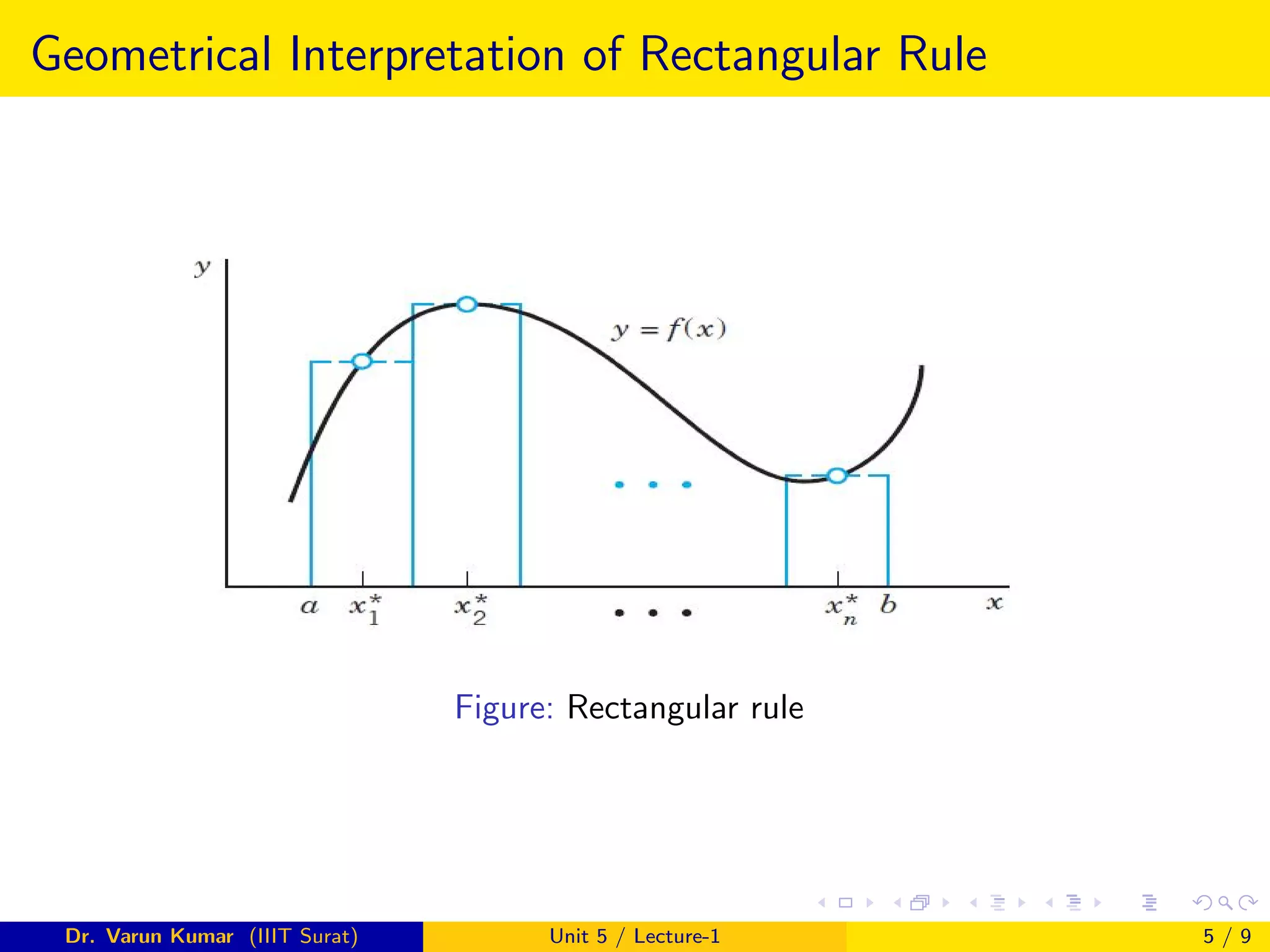
⇒ Rectangular rule is the simplest rule.
⇒ We divide the integration interval uniformly in n segments.
⇒ Let h is the resolution, where
h =
b − a
n
(2)
⇒ The definite integral of f (x) between the interval a ≤ x ≤ b is
J =
Z b
a
f (x)dx ≈ h[f (x∗
1 ) + f (x∗
2 ) + ..... + f (x∗
n )] (3)
Dr. Varun Kumar (IIIT Surat) Unit 5 / Lecture-1 4 / 9

5. Geometrical Interpretation of Rectangular Rule
Figure: Rectangular rule
Dr. Varun Kumar (IIIT Surat) Unit 5 / Lecture-1 5 / 9

6. Trapezoidal Rule
Key Points
⇒ The trapezoidal rule is generally more accurate.
⇒ Integral is obtained by the same subdivision as before.
⇒ Approximate f by a broken line of segments (chords) with endpoints
[a, f (a)], [x1, f (x1)], ...., [b, f (b)] on the curve of f (x).
⇒ Then the area under the curve of f between a and b is approximated
by n trapezoids of areas
1
2[f (a) + f (x1)]h, 1
2[f (x1) + f (x2)]h, ..... ,1
2[f (xn−1) + f (b)]h
Geometrical Interpretation of Trapezoidal Rule:
Dr. Varun Kumar (IIIT Surat) Unit 5 / Lecture-1 6 / 9

7. Continued–
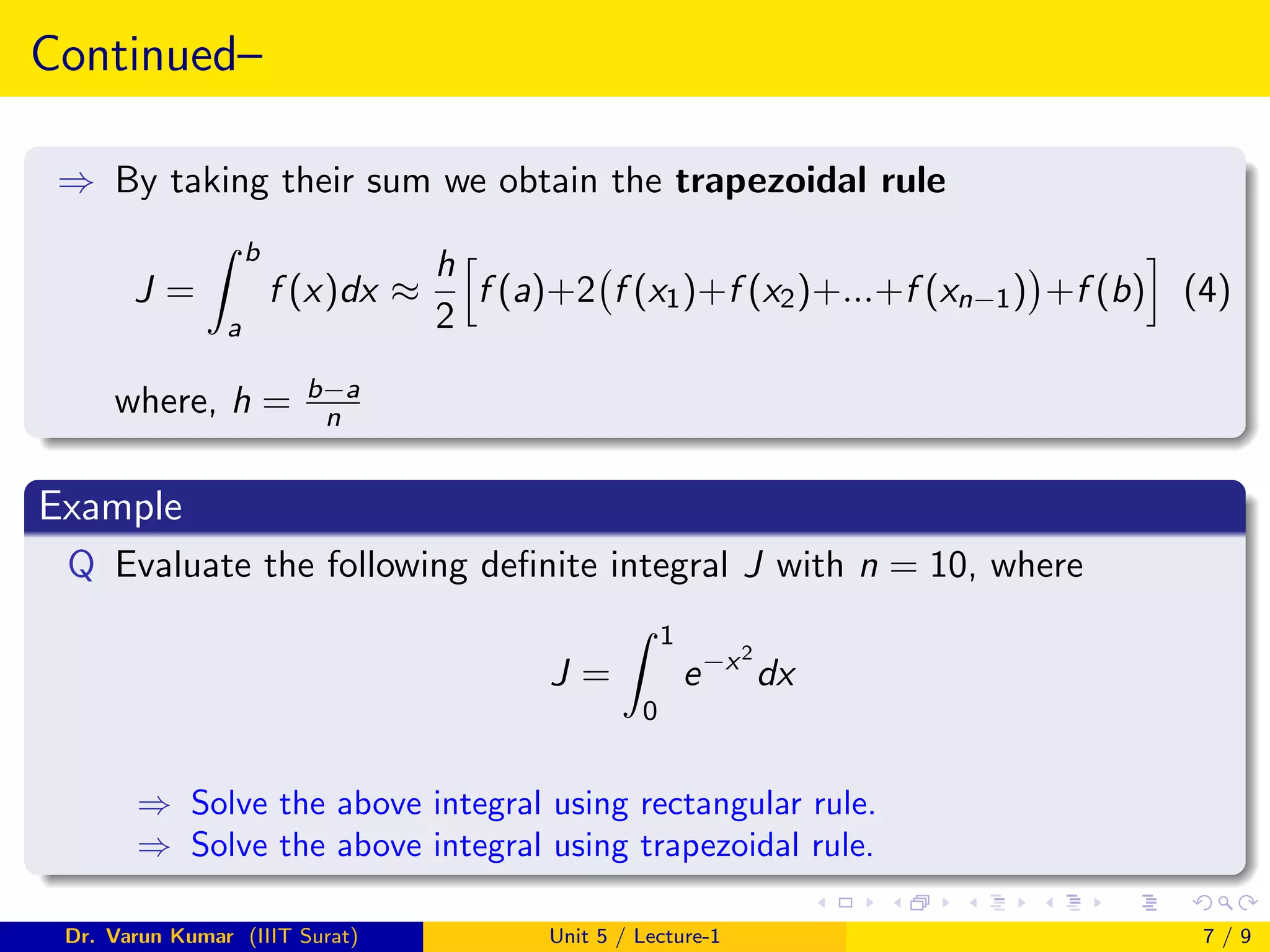
⇒ By taking their sum we obtain the trapezoidal rule
J =
Z b
a
f (x)dx ≈
h
2
h
f (a)+2 f (x1)+f (x2)+...+f (xn−1)
+f (b)
i
(4)
where, h = b−a
n
Example
Q Evaluate the following definite integral J with n = 10, where
J =
Z 1
0
e−x2
dx
⇒ Solve the above integral using rectangular rule.
⇒ Solve the above integral using trapezoidal rule.
Dr. Varun Kumar (IIIT Surat) Unit 5 / Lecture-1 7 / 9

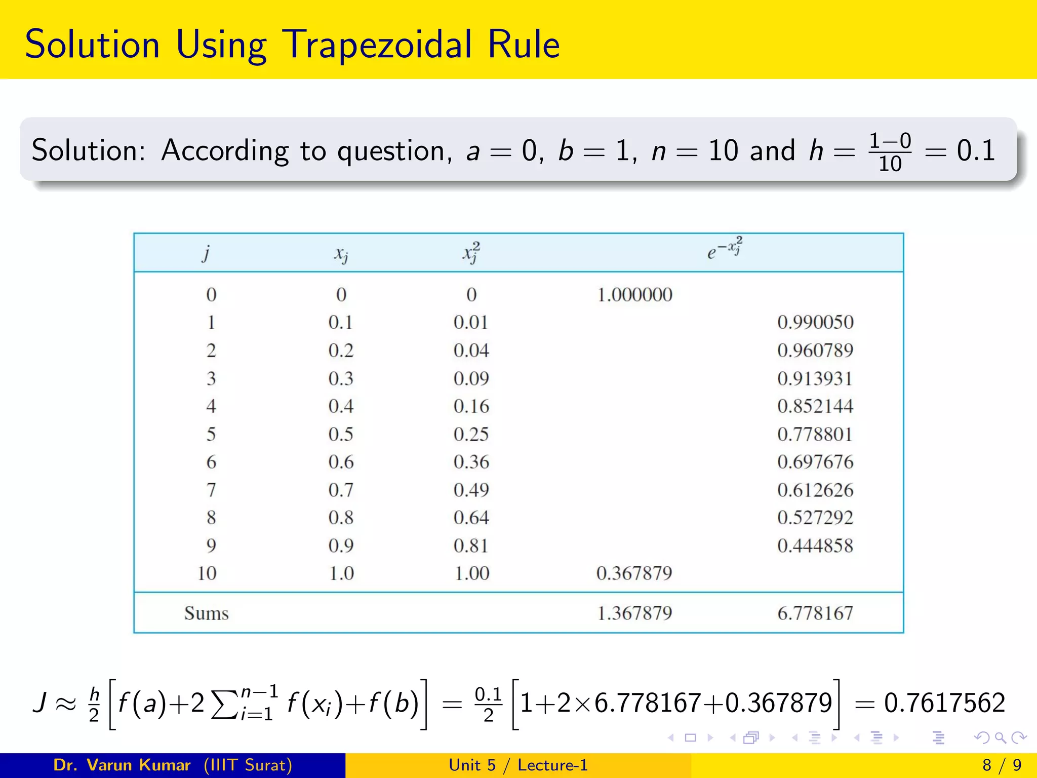
8. Solution Using Trapezoidal Rule
Solution: According to question, a = 0, b = 1, n = 10 and h = 1−0
10 = 0.1
J ≈ h
2
h
f (a)+2
Pn−1
i=1 f (xi )+f (b)
i
= 0.1
2
h
1+2×6.778167+0.367879
i
= 0.7617562
Dr. Varun Kumar (IIIT Surat) Unit 5 / Lecture-1 8 / 9

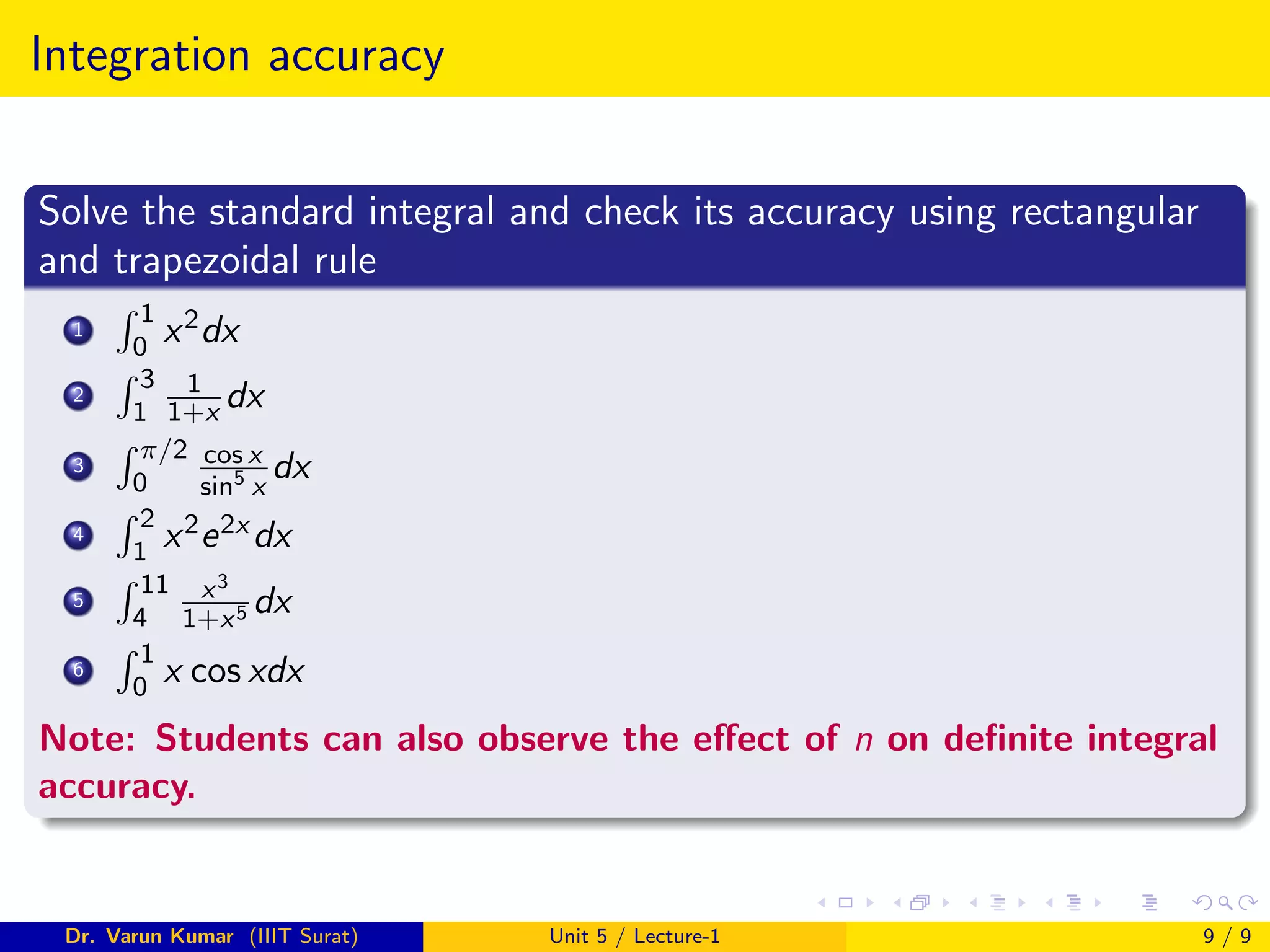
9. Integration accuracy
Solve the standard integral and check its accuracy using rectangular
and trapezoidal rule
1
R 1
0 x2dx
2
R 3
1
1
1+x dx
3
R π/2
0
cos x
sin5
x
dx
4
R 2
1 x2e2x dx
5
R 11
4
x3
1+x5 dx
6
R 1
0 x cos xdx
Note: Students can also observe the effect of n on definite integral
accuracy.
Dr. Varun Kumar (IIIT Surat) Unit 5 / Lecture-1 9 / 9