What is least-square fitting? Why it is done? How it is done?

1. Least Square
Fitting

2. Motivation
Humans’ natural instinct to find patterns

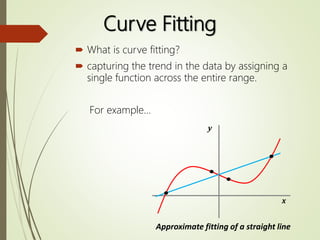
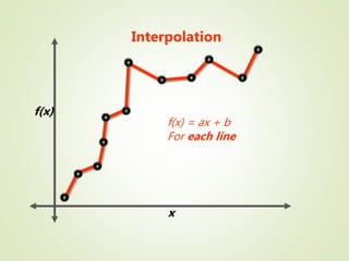
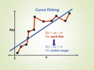
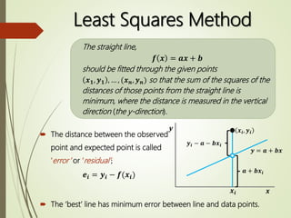
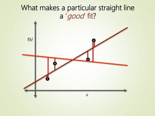
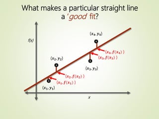
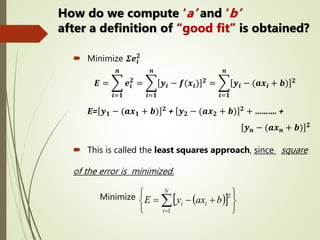
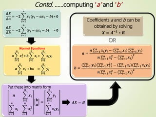
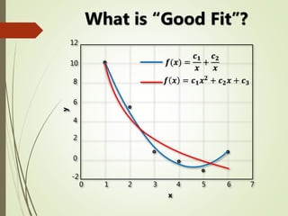
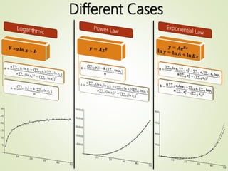
4. Introduction
 Least Square Methods (LSM) is probably the
most popular technique in statistics for
modelling.
 With applications in fields as diverse as
statistics, finance, medicines, economics &
psychology.
 Least squares is a way to use data to make
quantitative predictions.

5. History
Gauss
Legendre
First published by Legendre in 1805’s
paper ‘New Methods for Determination
of the Orbits of Comets’.
In 1809, Gauss published a memoir in
which he mentioned that he had
previously discovered LSM and it as
early as 1795 in estimating the orbit of
an asteroid.
Both Gauss and Legendre used the
method of least squares to understand
the orbits of comets, based on inexact
measurements of the comets’ previous
locations.

6. Curve Fitting
 What is curve fitting?
 capturing the trend in the data by assigning a
single function across the entire range.
For example…
x
y
Approximate fitting of a straight line

7. f(x) = ax + b
For each line
Interpolation
x
f(x)

8. f(x) = ax + b
For each line
Curve Fitting
f(x) = ax + b
For entire range
x
f(x)

9. The straight line,
𝒇 𝒙 = 𝒂𝒙 + 𝒃
should be fitted through the given points
𝒙 𝟏, 𝒚 𝟏 , … , (𝒙 𝒏, 𝒚 𝒏) so that the sum of the squares of the
distances of those points from the straight line is
minimum, where the distance is measured in the vertical
direction (the y-direction).
 The distance between the observed
point and expected point is called
‘error’ or ‘residual’;
𝒆𝒊 = 𝒚𝒊 − 𝒇(𝒙𝒊)
Least Squares Method
 The ‘best’ line has minimum error between line and data points.
x
y 𝒙𝒊, 𝒚𝒊
𝒚𝒊 − 𝒂 − 𝒃𝒙𝒊
𝒂 + 𝒃𝒙𝒊
𝒚 = 𝒂 + 𝒃𝒙
𝒙𝒊

10. x
f(x)
What makes a particular straight line
a ‘good’ fit?

11. (𝒙 𝟐, 𝒚 𝟐)
(𝒙 𝟒, 𝒚 𝟒)
(𝒙 𝟏, 𝒚 𝟏)
(𝒙 𝟑, 𝒚 𝟑)
(𝒙 𝟏, 𝒇(𝒙 𝟏) )
(𝒙 𝟐, 𝒇(𝒙 𝟐) )
(𝒙 𝟑, 𝒇(𝒙 𝟑) )
(𝒙 𝟒, 𝒇(𝒙 𝟒) )
x
f(x)
What makes a particular straight line
a ‘good’ fit?

12.  Minimize 𝜮𝒆𝒊
𝟐
𝑬 =
𝒊=𝟏
𝒏
𝒆𝒊
𝟐
=
𝒊=𝟏
𝒏
𝒚𝒊 − 𝒇(𝒙𝒊) 𝟐 =
𝒊=𝟏
𝒏
𝒚𝒊 − (𝒂𝒙𝒊 + 𝒃) 𝟐
E= 𝒚 𝟏 − (𝒂𝒙 𝟏 + 𝒃) 𝟐
+ 𝒚 𝟐 − (𝒂𝒙 𝟐 + 𝒃) 𝟐
+ ………. +
𝒚 𝒏 − (𝒂𝒙 𝒏 + 𝒃) 𝟐
 This is called the least squares approach, since square
of the error is minimized.
How do we compute ‘a’ and ‘b’
after a definition of “good fit” is obtained?
  






 
N
i
ii baxyE
1
2Minimize

13. Contd. ……computing ‘a’ and ‘b’
𝝏𝑬
𝝏𝒂
= −𝟐
𝒊=𝟏
𝒏
𝒙𝒊 (𝒚𝒊 − 𝒂𝒙𝒊 − 𝒃) = 0
𝝏𝑬
𝝏𝒃
= −𝟐
𝒊=𝟏
𝒏
(𝒚𝒊 − 𝒂𝒙𝒊 − 𝒃) = 0
Normal Equations
𝒂
𝒊=𝟏
𝒏
𝒙𝒊
𝟐
+ 𝒃
𝒊=𝟏
𝒏
𝒙𝒊 =
𝒊=𝟏
𝒏
𝒙𝒊 𝒚𝒊
𝒂
𝒊=𝟏
𝒏
𝒙𝒊 + 𝒃 𝒏 =
𝒊=𝟏
𝒏
𝒚𝒊
Put these into matrix form
𝒏
𝒊=𝟏
𝒏
𝒙𝒊
𝒊=𝟏
𝒏
𝒙𝒊
𝒊=𝟏
𝒏
𝒙𝒊
𝟐
𝒃
𝒂
= 𝒊=𝟏
𝒏
𝒚𝒊
𝒊=𝟏
𝒏
𝒙𝒊 𝒚𝒊
𝑨𝑿 = 𝑩
Coefficients a and b can be
obtained by solving
𝑿 = 𝑨−𝟏 ∗ 𝑩
𝒂 =
𝒏 𝒊=𝟏
𝒏
𝒙𝒊 𝒚𝒊 − 𝒊=𝟏
𝒏
𝒙𝒊 𝒊=𝟏
𝒏
𝒚𝒊
𝒏 𝒊=𝟏
𝒏
𝒙𝒊
𝟐
− 𝒊=𝟏
𝒏
𝒙𝒊
𝟐
𝒃 =
𝒊=𝟏
𝒏
𝒚𝒊 𝒊=𝟏
𝒏
𝒙𝒊
𝟐
− 𝒊=𝟏
𝒏
𝒙𝒊 𝒊=𝟏
𝒏
𝒙𝒊 𝒚𝒊
𝒏 𝒊=𝟏
𝒏
𝒙𝒊
𝟐
− 𝒊=𝟏
𝒏
𝒙𝒊
𝟐

14. 0 1 2 3 4 5 6 7
x
12
10
8
6
4
2
0
-2
y
What is “Good Fit”?
𝒇(𝒙) =
𝒄 𝟏
𝒙
+
𝒄 𝟐
𝒙
𝒇 𝒙 = 𝒄 𝟏 𝒙 𝟐
+ 𝒄 𝟐 𝒙 + 𝒄 𝟑

15. The Least-Squares mth Degree
Polynomials
 Using a polynomial of degree m
𝒚 = 𝒂 𝟎 + 𝒂 𝟏 𝒙 + 𝒂 𝟐 𝒙 𝟐
+ ⋯ + 𝒂 𝒎 𝒙 𝒎
 To approx. given set of data 𝒙 𝟏, 𝒚 𝟏 , 𝒙 𝟐, 𝒚 𝟐 , … , (𝒙 𝒏, 𝒚 𝒏) where
𝒎 ≤ 𝒏 − 𝟏, the best fitting curve has the least square error, i.e.,
𝑴𝒊𝒏𝒊𝒎𝒊𝒛𝒆{𝑬 =
𝒊=𝟏
𝒏
{𝒚𝒊 − 𝒇(𝒙𝒊)} 𝟐
}
𝑬 =
𝒊=𝟏
𝒏
{𝒚𝒊 − 𝒂 𝟎 + 𝒂 𝟏 𝒙𝒊 + 𝒂 𝟐 𝒙𝒊
𝟐
+ ⋯ + 𝒂 𝒎 𝒙𝒊
𝒎
} 𝟐
 Obtain normal equations
𝝏𝑬
𝝏𝒂 𝟎
= 𝟎,
𝝏𝑬
𝝏𝒂 𝟏
= 𝟎, … . ,
𝝏𝑬
𝝏𝒂 𝒎
= 𝟎
 The normal equations can be put in matrix form
𝑨𝑿 = 𝑩 which can be solved to get 𝑿 = 𝑨−𝟏 ∗ B

16. Fitting a Second Degree
(Parabola) Polynomial
 Parabolic Trend is given by 𝒚 = 𝒂 𝟎 + 𝒂 𝟏 𝒙 + 𝒂 𝟐 𝒙 𝟐
 Then error is; 𝑬 = (𝒚 − (𝒂 𝟎+𝒂 𝟏 𝒙 + 𝒂 𝟐 𝒙 𝟐))
𝟐
 Minimizing

𝝏𝑬
𝝏𝒂 𝟎
= 𝟎 = −𝟐 (𝒚 − 𝒂 𝟎 + 𝒂 𝟏 𝒙 + 𝒂 𝟐 𝒙 𝟐
)

𝝏𝑬
𝝏𝒂 𝟏
= 𝟎 = −𝟐 𝒙(𝒚 − 𝒂 𝟎 + 𝒂 𝟏 𝒙 + 𝒂 𝟐 𝒙 𝟐)

𝝏𝑬
𝝏𝒂 𝟐
= 𝟎 = −𝟐 𝒙 𝟐(𝒚 − 𝒂 𝟎 + 𝒂 𝟏 𝒙 + 𝒂 𝟐 𝒙 𝟐)
 Normal equations are
 𝒚 = 𝒏𝒂 𝟎 + 𝒂 𝟏 𝒕 + 𝒂 𝟐 𝒙 𝟐
 𝒙𝒚 = 𝒂 𝟎 𝒙 + 𝒂 𝟏 𝒙 𝟐
+ 𝒂 𝟐 𝒙 𝟑
 𝒙 𝟐
𝒚 = 𝒂 𝟎 𝒙 𝟐
+ 𝒂 𝟏 𝒙 𝟑
+ 𝒂 𝟑 𝒙 𝟒

17. Different Cases

18. Limitations
 Most serious limitation: The determination of the
type of the trend curve to be fitted, whether we
should fit a linear or a parabolic trend or some
other more complicated trend curve.
 The addition of single new observation
necessitates all the calculations to be done
afresh.
 This method requires more calculations and
quite tedious and time consuming as compared
with other methods.

19.  If P is the pull required to pull the load W by means of a pulley
block, find a linear law of the form P=mW+ c connecting P and
W (in kg.wt), using the following data
Compute P when W=150 kg.wt
 Sol- The corresponding normal Equations are
𝑃 = 4𝑐 + 𝑚 𝑊 ; 𝑊𝑃 = 𝑐 𝑊 + 𝑚 𝑊2
P= 12 15 21 25
W=50 70 100 120
W P W² WP
50
70
100
120
12
15
21
25
2500
4900
10000
14400
600
1050
2100
3000
Total =340 73 31800 6750
Example

20.  Substituting the values
73 = 4c + 340m ;
6750 = 340c + 31800m
Example contd…
 With little algebra,
we get
m = 0.1879 & c = 2.2785
Hence the line if best fit is
P = 2.2759 + 0.1879 W
When W= 150 kg,
P= 2.2785 + 0.1879 X 150 = 30.4635
0
5
10
15
20
25
30
0 50 100 150
P
W
P vs W
P
0
5
10
15
20
25
30
0 50 100 150
P
W
P vs W
P(expected)

21. References
 https://priceonomics.com/the-discovery-of-statistical-regression/
 http://web.iitd.ac.in/~pmvs/courses/mel705/curvefitting.pdf
 Least Squares Fitting of Data to a Curve/ Gerald Recktenwald/
Portland State University/ Department of Mechanical Engineering
 Fundamentals of Statistics, S.C. Gupta
 Higher Engineering Methods, Dr. B.S. Grewal
 Advanced Engineering Method, ERWIN KREYSZIG
 http://mathworld.wolfram.com/LeastSquaresFittingLogarithmic.htm
l
 http://mathworld.wolfram.com/LeastSquaresFittingExponential.html
 http://mathworld.wolfram.com/LeastSquaresFittingPowerLaw.html

22. Thank You