1
PRESENTATION ON INTRODUCTION
TO SEVERAL VARIABLES AND
PARTIAL DERIVATIVES
2
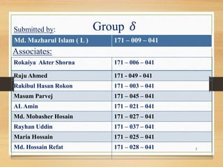
Rokaiya Akter Shorna 171 – 006 – 041
Raju Ahmed 171 - 049 - 041
Rakibul Hasan Rokon 171 – 003 – 041
Masum Parvej 171 – 045 – 041
ALAmin 171 – 021 – 041
Md. Mobasher Hosain 171 – 027 – 041
Rayhan Uddin 171 – 037 – 041
Maria Hossain 171 – 025 – 041
Md. Hossain Refat 171 – 028 – 041
Associates:
Submitted by:
Md. Mazharul Islam ( L ) 171 – 009 – 041
Group 𝛿
SUBMITTED TO
3
A.B.M Minhajur Rahman
Lecturer of Mathematics
Department of Basic Science
Primeasia University , Banani
Chapter 01
Introduction to several
variables
4
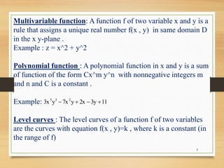
Multivariable function: A function f of two variable x and y is a
rule that assigns a unique real number f(x , y) in same domain D
in the x y-plane .
Example : z = x^2 + y^2
Polynomial function : A polynomial function in x and y is a sum
of function of the form Cx^m y^n with nonnegative integers m
and n and C is a constant .
Example:
Level curves : The level curves of a function f of two variables
are the curves with equation f(x , y)=k , where k is a constant (in
the range of f)
113y2xy7xy3x 235

5
6
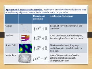
Application of multivariable function : Techniques of multivariable calculus are used
to study many objects of interest in the material world. In particular
Domain and
codomain
Application Techniques
Curves Length of curves line integrals and
curvature
Surface Areas of surfaces, surface integrals,
flux through surfaces, and curvature.
Scalar field Maxima and minima, Lagrange
multipliers, directional derivatives,
level sets.
Vector field Any of the operations of vector
calculus including gradient,
divergence, and curl.
7
Example 01 : Find the domain and range of g(x , y) = 9 − đ‘„2 − 𝑩2
Solve: Now the domain of this function
D ={(x , y) | 9 − đ‘„2
− 𝑩2
≄ 0 }
= {(x , y) | đ‘„2
+ 𝑩2
≀ 9 }
Which is the disk with center (0 , 0) and radius 3
The range of g is
{ z | z = 9 − đ‘„2 − 𝑩2 , (x , y) ∈ D }
Since z is positive square root , z ≄ 0
So the range is = { z | 0 ≀ z ≀ 3 }
= [0 , 3]
8
Example 02 : Find the domain and range of g(x , y) = 9 − đ‘„2 − 4𝑩2
Solve: Now the domain of this function
D ={(x , y) | 9 − đ‘„2
− 4𝑩2
≄ 0 }
= {(x , y) | đ‘„2
+ 4𝑩2
≀ 9 }
= {(x , y) | đ‘„2/32 + 𝑩2/
3
2
2
= 1 }
Which is the disk with center (3 , 3/2 )
The range of g is
{ z | z = 9 − đ‘„2 − 4𝑩2 , (x , y) ∈ D }
Since z is positive square root , z ≄ 0
So the range is = { z | 0 ≀ z ≀ 3 }
= [0 , 3]
9
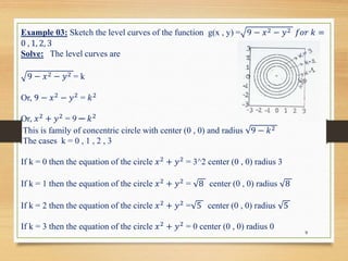
Example 03: Sketch the level curves of the function g(x , y) = 9 − đ‘„2 − 𝑩2 𝑓𝑜𝑟 𝑘 =
0 , 1, 2, 3
Solve: The level curves are
9 − đ‘„2 − 𝑩2 = k
Or, 9 − đ‘„2
− 𝑩2
= 𝑘2
Or, đ‘„2
+ 𝑩2
= 9 ─ 𝑘2
This is family of concentric circle with center (0 , 0) and radius 9 − 𝑘2
The cases k = 0 , 1 , 2 , 3
If k = 0 then the equation of the circle đ‘„2
+ 𝑩2
= 3^2 center (0 , 0) radius 3
If k = 1 then the equation of the circle đ‘„2
+ 𝑩2
= 8 center (0 , 0) radius 8
If k = 2 then the equation of the circle đ‘„2
+ 𝑩2
= 5 center (0 , 0) radius 5
If k = 3 then the equation of the circle đ‘„2
+ 𝑩2
= 0 center (0 , 0) radius 0
10
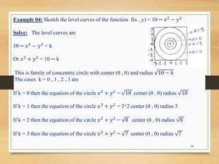
Example 04: Sketch the level curves of the function f(x , y) = 10 ─ đ‘„2
− 𝑩2
Solve: The level curves are
10 ─ đ‘„2
− 𝑩2
= k
Or đ‘„2
+ 𝑩2
= 10 ─ k
This is family of concentric circle with center (0 , 0) and radius 10 − 𝑘
The cases k = 0 , 1 , 2 , 3 are
If k = 0 then the equation of the circle đ‘„2 + 𝑩2 = 10 center (0 , 0) radius 10
If k = 1 then the equation of the circle đ‘„2
+ 𝑩2
= 3^2 center (0 , 0) radius 3
If k = 2 then the equation of the circle đ‘„2
+ 𝑩2
= 8 center (0 , 0) radius 8
If k = 3 then the equation of the circle đ‘„2 + 𝑩2 = 7 center (0 , 0) radius 7
Chapter 04
Partial derivatives
11
12
Partial derivatives
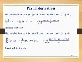
The partial derivative of f(x , y) with respect to x at the point (xₒ , yₒ) is ,
𝜕𝑓
đœ•đ‘„
⃒ đ‘„â‚’ , 𝑩ₒ =
𝑑
đ‘‘đ‘„
f(x , yₒ)⃒x=xₒ =lim
ℎ→0
𝑓 đ‘„â‚’+ℎ ,𝑩ₒ −𝑓(đ‘„â‚’ ,𝑩ₒ)
ℎ
Provided limit exist
The partial derivative of f(x , y) with respect to x at the point (xₒ , yₒ) is ,
𝜕𝑓
𝜕𝑩
⃒ đ‘„â‚’ , 𝑩ₒ =
𝑑
𝑑𝑩
f(xₒ , y)⃒y=yₒ =lim
ℎ→0
𝑓 đ‘„â‚’ ,𝑩ₒ+ℎ −𝑓(đ‘„â‚’ ,𝑩ₒ)
ℎ
Provided limit exist
13
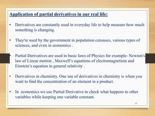
Application of partial derivatives in our real life:
‱ Derivatives are constantly used in everyday life to help measure how much
something is changing.
‱ They're used by the government in population censuses, various types of
sciences, and even in economics .
‱ Partial Derivatives are used in basic laws of Physics for example- Newton's
law of Linear motion , Maxwell’s equations of electromagnetism and
Einstein’s equation in general relativity .
‱ Derivatives in chemistry. One use of derivatives in chemistry is when you
want to find the concentration of an element in a product.
‱ In economics we use Partial Derivative to check what happens to other
variables while keeping one variable constant.
14
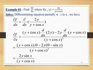
Example 01 : Find
𝜕𝑓
đœ•đ‘„
where f(x , y) =
2𝑩
𝑩+đ‘đ‘œđ‘ đ‘„
Solve: Differentiating equation partially w . r to x , we have
)cos(
sin2
)cos(
)sin0(20).cos(
)cos(
)cos(2)2()cos(
)
cos
2
(
2
2
xy
xy
xy
xyxy
xy
xy
dx
d
yy
dx
d
xy
x
f
xy
y
dxdx
f














15
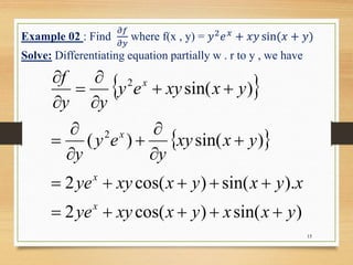
Example 02 : Find
𝜕𝑓
𝜕𝑩
where f(x , y) = 𝑩2 𝑒 đ‘„ + đ‘„đ‘Š sin(đ‘„ + 𝑩)
Solve: Differentiating equation partially w . r to y , we have
 
 
)sin()cos(2
).sin()cos(2
)sin()(
)sin(
2
2
yxxyxxyye
xyxyxxyye
yxxy
y
ey
y
yxxyey
yy
f
x
x
x
x















16
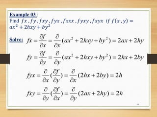
Example 03 :
Find đ‘“đ‘„ , 𝑓𝑩 , đ‘“đ‘„đ‘Š , đ‘“đ‘Šđ‘„ , đ‘“đ‘„đ‘„đ‘„ , đ‘“đ‘Šđ‘„đ‘Š , đ‘“đ‘„đ‘Šđ‘„ 𝑖𝑓 𝑓 đ‘„ , 𝑩 =
đ‘Žđ‘„2 + 2â„Žđ‘„đ‘Š + 𝑏𝑩2
Solve:
hhyax
yx
f
y
fxy
hbyhx
xy
f
x
fyx
byhxbyhxyax
yy
f
fy
hyaxbyhxyax
xx
f
fx
2)22()(
2)22()(
22)2(
22)2(
22
22
































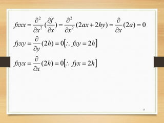
17
 
 hfyxh
x
fxyx
hfxyh
y
fyxy
a
x
hyax
xx
f
x
fxxx
20)2(
20)2(
0)2()22()( 2
2
2
2




















18
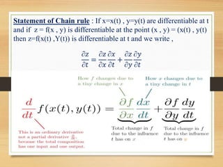
Statement of Chain rule : If x=x(t) , y=y(t) are differentiable at t
and if z = f(x , y) is differentiable at the point (x , y) = (x(t) , y(t)
then z=f(x(t) ,Y(t)) is differentiable at t and we write ,
∂𝑧
∂𝑡
=
∂𝑧
âˆ‚đ‘„
âˆ‚đ‘„
∂𝑡
+
∂𝑧
∂𝑩
∂𝑩
∂𝑡
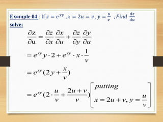
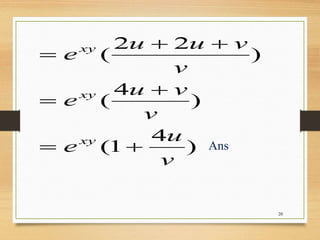
Example 04 : If 𝑧 = 𝑒 đ‘„đ‘Š , đ‘„ = 2𝑱 = 𝑣 , 𝑩 =
𝑱
𝑣
, đč𝑖𝑛𝑑
𝑑𝑧
𝑑𝑱
solve:
ïƒș
ïƒș

ïƒč
ïƒȘ
ïƒȘ



















v
u
yvux
putting
v
vu
v
u
e
v
x
ye
v
xeye
u
y
y
z
u
x
x
z
xy
xy
xyxy
,2
)
2
2(
)2(
1
2
u
z
20
)
4
1(
)
4
(
)
22
(
v
u
e
v
vu
e
v
vuu
e
xy
xy
xy





Ans
21

PRESENTATION ON INTRODUCTION TO SEVERAL VARIABLES AND PARTIAL DERIVATIVES

  • 1.
    1 PRESENTATION ON INTRODUCTION TOSEVERAL VARIABLES AND PARTIAL DERIVATIVES
  • 2.
    2 Rokaiya Akter Shorna171 – 006 – 041 Raju Ahmed 171 - 049 - 041 Rakibul Hasan Rokon 171 – 003 – 041 Masum Parvej 171 – 045 – 041 ALAmin 171 – 021 – 041 Md. Mobasher Hosain 171 – 027 – 041 Rayhan Uddin 171 – 037 – 041 Maria Hossain 171 – 025 – 041 Md. Hossain Refat 171 – 028 – 041 Associates: Submitted by: Md. Mazharul Islam ( L ) 171 – 009 – 041 Group 𝛿
  • 3.
    SUBMITTED TO 3 A.B.M MinhajurRahman Lecturer of Mathematics Department of Basic Science Primeasia University , Banani
  • 4.
    Chapter 01 Introduction toseveral variables 4
  • 5.
    Multivariable function: Afunction f of two variable x and y is a rule that assigns a unique real number f(x , y) in same domain D in the x y-plane . Example : z = x^2 + y^2 Polynomial function : A polynomial function in x and y is a sum of function of the form Cx^m y^n with nonnegative integers m and n and C is a constant . Example: Level curves : The level curves of a function f of two variables are the curves with equation f(x , y)=k , where k is a constant (in the range of f) 113y2xy7xy3x 235  5
  • 6.
    6 Application of multivariablefunction : Techniques of multivariable calculus are used to study many objects of interest in the material world. In particular Domain and codomain Application Techniques Curves Length of curves line integrals and curvature Surface Areas of surfaces, surface integrals, flux through surfaces, and curvature. Scalar field Maxima and minima, Lagrange multipliers, directional derivatives, level sets. Vector field Any of the operations of vector calculus including gradient, divergence, and curl.
  • 7.
    7 Example 01 :Find the domain and range of g(x , y) = 9 − đ‘„2 − 𝑩2 Solve: Now the domain of this function D ={(x , y) | 9 − đ‘„2 − 𝑩2 ≄ 0 } = {(x , y) | đ‘„2 + 𝑩2 ≀ 9 } Which is the disk with center (0 , 0) and radius 3 The range of g is { z | z = 9 − đ‘„2 − 𝑩2 , (x , y) ∈ D } Since z is positive square root , z ≄ 0 So the range is = { z | 0 ≀ z ≀ 3 } = [0 , 3]
  • 8.
    8 Example 02 :Find the domain and range of g(x , y) = 9 − đ‘„2 − 4𝑩2 Solve: Now the domain of this function D ={(x , y) | 9 − đ‘„2 − 4𝑩2 ≄ 0 } = {(x , y) | đ‘„2 + 4𝑩2 ≀ 9 } = {(x , y) | đ‘„2/32 + 𝑩2/ 3 2 2 = 1 } Which is the disk with center (3 , 3/2 ) The range of g is { z | z = 9 − đ‘„2 − 4𝑩2 , (x , y) ∈ D } Since z is positive square root , z ≄ 0 So the range is = { z | 0 ≀ z ≀ 3 } = [0 , 3]
  • 9.
    9 Example 03: Sketchthe level curves of the function g(x , y) = 9 − đ‘„2 − 𝑩2 𝑓𝑜𝑟 𝑘 = 0 , 1, 2, 3 Solve: The level curves are 9 − đ‘„2 − 𝑩2 = k Or, 9 − đ‘„2 − 𝑩2 = 𝑘2 Or, đ‘„2 + 𝑩2 = 9 ─ 𝑘2 This is family of concentric circle with center (0 , 0) and radius 9 − 𝑘2 The cases k = 0 , 1 , 2 , 3 If k = 0 then the equation of the circle đ‘„2 + 𝑩2 = 3^2 center (0 , 0) radius 3 If k = 1 then the equation of the circle đ‘„2 + 𝑩2 = 8 center (0 , 0) radius 8 If k = 2 then the equation of the circle đ‘„2 + 𝑩2 = 5 center (0 , 0) radius 5 If k = 3 then the equation of the circle đ‘„2 + 𝑩2 = 0 center (0 , 0) radius 0
  • 10.
    10 Example 04: Sketchthe level curves of the function f(x , y) = 10 ─ đ‘„2 − 𝑩2 Solve: The level curves are 10 ─ đ‘„2 − 𝑩2 = k Or đ‘„2 + 𝑩2 = 10 ─ k This is family of concentric circle with center (0 , 0) and radius 10 − 𝑘 The cases k = 0 , 1 , 2 , 3 are If k = 0 then the equation of the circle đ‘„2 + 𝑩2 = 10 center (0 , 0) radius 10 If k = 1 then the equation of the circle đ‘„2 + 𝑩2 = 3^2 center (0 , 0) radius 3 If k = 2 then the equation of the circle đ‘„2 + 𝑩2 = 8 center (0 , 0) radius 8 If k = 3 then the equation of the circle đ‘„2 + 𝑩2 = 7 center (0 , 0) radius 7
  • 11.
  • 12.
    12 Partial derivatives The partialderivative of f(x , y) with respect to x at the point (xₒ , yₒ) is , 𝜕𝑓 đœ•đ‘„ ⃒ đ‘„â‚’ , 𝑩ₒ = 𝑑 đ‘‘đ‘„ f(x , yₒ)⃒x=xₒ =lim ℎ→0 𝑓 đ‘„â‚’+ℎ ,𝑩ₒ −𝑓(đ‘„â‚’ ,𝑩ₒ) ℎ Provided limit exist The partial derivative of f(x , y) with respect to x at the point (xₒ , yₒ) is , 𝜕𝑓 𝜕𝑩 ⃒ đ‘„â‚’ , 𝑩ₒ = 𝑑 𝑑𝑩 f(xₒ , y)⃒y=yₒ =lim ℎ→0 𝑓 đ‘„â‚’ ,𝑩ₒ+ℎ −𝑓(đ‘„â‚’ ,𝑩ₒ) ℎ Provided limit exist
  • 13.
    13 Application of partialderivatives in our real life: ‱ Derivatives are constantly used in everyday life to help measure how much something is changing. ‱ They're used by the government in population censuses, various types of sciences, and even in economics . ‱ Partial Derivatives are used in basic laws of Physics for example- Newton's law of Linear motion , Maxwell’s equations of electromagnetism and Einstein’s equation in general relativity . ‱ Derivatives in chemistry. One use of derivatives in chemistry is when you want to find the concentration of an element in a product. ‱ In economics we use Partial Derivative to check what happens to other variables while keeping one variable constant.
  • 14.
    14 Example 01 :Find 𝜕𝑓 đœ•đ‘„ where f(x , y) = 2𝑩 𝑩+đ‘đ‘œđ‘ đ‘„ Solve: Differentiating equation partially w . r to x , we have )cos( sin2 )cos( )sin0(20).cos( )cos( )cos(2)2()cos( ) cos 2 ( 2 2 xy xy xy xyxy xy xy dx d yy dx d xy x f xy y dxdx f              
  • 15.
    15 Example 02 :Find 𝜕𝑓 𝜕𝑩 where f(x , y) = 𝑩2 𝑒 đ‘„ + đ‘„đ‘Š sin(đ‘„ + 𝑩) Solve: Differentiating equation partially w . r to y , we have     )sin()cos(2 ).sin()cos(2 )sin()( )sin( 2 2 yxxyxxyye xyxyxxyye yxxy y ey y yxxyey yy f x x x x               
  • 16.
    16 Example 03 : Findđ‘“đ‘„ , 𝑓𝑩 , đ‘“đ‘„đ‘Š , đ‘“đ‘Šđ‘„ , đ‘“đ‘„đ‘„đ‘„ , đ‘“đ‘Šđ‘„đ‘Š , đ‘“đ‘„đ‘Šđ‘„ 𝑖𝑓 𝑓 đ‘„ , 𝑩 = đ‘Žđ‘„2 + 2â„Žđ‘„đ‘Š + 𝑏𝑩2 Solve: hhyax yx f y fxy hbyhx xy f x fyx byhxbyhxyax yy f fy hyaxbyhxyax xx f fx 2)22()( 2)22()( 22)2( 22)2( 22 22                                
  • 17.
    17    hfyxh x fxyx hfxyh y fyxy a x hyax xx f x fxxx 20)2( 20)2( 0)2()22()(2 2 2 2                    
  • 18.
    18 Statement of Chainrule : If x=x(t) , y=y(t) are differentiable at t and if z = f(x , y) is differentiable at the point (x , y) = (x(t) , y(t) then z=f(x(t) ,Y(t)) is differentiable at t and we write , ∂𝑧 ∂𝑡 = ∂𝑧 âˆ‚đ‘„ âˆ‚đ‘„ ∂𝑡 + ∂𝑧 ∂𝑩 ∂𝑩 ∂𝑡
  • 19.
    Example 04 :If 𝑧 = 𝑒 đ‘„đ‘Š , đ‘„ = 2𝑱 = 𝑣 , 𝑩 = 𝑱 𝑣 , đč𝑖𝑛𝑑 𝑑𝑧 𝑑𝑱 solve: ïƒș ïƒș  ïƒč ïƒȘ ïƒȘ                    v u yvux putting v vu v u e v x ye v xeye u y y z u x x z xy xy xyxy ,2 ) 2 2( )2( 1 2 u z
  • 20.
  • 21.