Download as PDF, PPTX

![Shortest-Paths Idea
● d(u,v) length of the shortest path from u to v.
● All SSSP algorithms maintain a field d[u] for every vertex
u. d[u] will be an estimate of d(s,u). As the algorithm
progresses, we will refine d[u] until, at termination,
d[u] = d(s,u). Whenever we discover a new shortest path to
u, we update d[u].
● In fact, d[u] will always be an overestimate of d(s,u):
● d[u] d(s,u)
● We’ll use p[u] to point to the parent (or predecessor) of u on
the shortest path from s to u. We update p[u] when we
update d[u].](https://image.slidesharecdn.com/lecture17-140420071825-phpapp02/75/Shortest-Path-in-Graph-8-2048.jpg)
![SSSP Subroutine
RELAX(u, v, w)
> (Maybe) improve our estimate of the distance to v
> by considering a path along the edge (u, v).
if d[u] + w(u, v) < d[v] then
d[v] d[u] + w(u, v) > actually, DECREASE-KEY
p[v] u > remember predecessor on path
u v
w(u,v)
d[v]d[u]](https://image.slidesharecdn.com/lecture17-140420071825-phpapp02/75/Shortest-Path-in-Graph-9-2048.jpg)
![Dijkstra’s Algorithm
● Assume that all edge weights are 0.
● Idea: say we have a set K containing all
vertices whose shortest paths from s are
known
(i.e. d[u] = d(s,u) for all u in K).
● Now look at the “frontier” of K—all vertices
adjacent to a vertex in K. the rest
of the
graph
s
K](https://image.slidesharecdn.com/lecture17-140420071825-phpapp02/75/Shortest-Path-in-Graph-10-2048.jpg)
![Dijkstra’s: Theorem
● At each frontier
vertex u, update d[u]
to be the minimum
from all edges from
K.
● Now pick the frontier
vertex u with the
smallest value of
d[u].
● Claim: d[u] = d(s,u)
s
4
9
6
6
2
1
3
8
min(4+2, 6+1) = 6
min(4+8, 6+3) = 9](https://image.slidesharecdn.com/lecture17-140420071825-phpapp02/75/Shortest-Path-in-Graph-11-2048.jpg)


![Code for Dijkstra’s Algorithm
1 DIJKSTRA(G, w, s) > Graph, weights, start vertex
2 for each vertex v in V[G] do
3 d[v]
4 p[v] NIL
5 d[s] 0
6 Q BUILD-PRIORITY-QUEUE(V[G])
7 > Q is V[G] - K
8 while Q is not empty do
9 u = EXTRACT-MIN(Q)
10 for each vertex v in Adj[u]
11 RELAX(u, v, w) // DECREASE_KEY](https://image.slidesharecdn.com/lecture17-140420071825-phpapp02/75/Shortest-Path-in-Graph-22-2048.jpg)

![Bellman-Ford: Idea
● Repeatedly update d for all pairs of vertices
connected by an edge.
● Theorem: If u and v are two vertices with an
edge from u to v, and s u v is a shortest
path, and d[u] = d(s,u),
● then d[u]+w(u,v) is the length of a shortest
path to v.
● Proof: Since s u v is a shortest path, its
length is d(s,u) + w(u,v) = d[u] + w(u,v). ](https://image.slidesharecdn.com/lecture17-140420071825-phpapp02/75/Shortest-Path-in-Graph-26-2048.jpg)
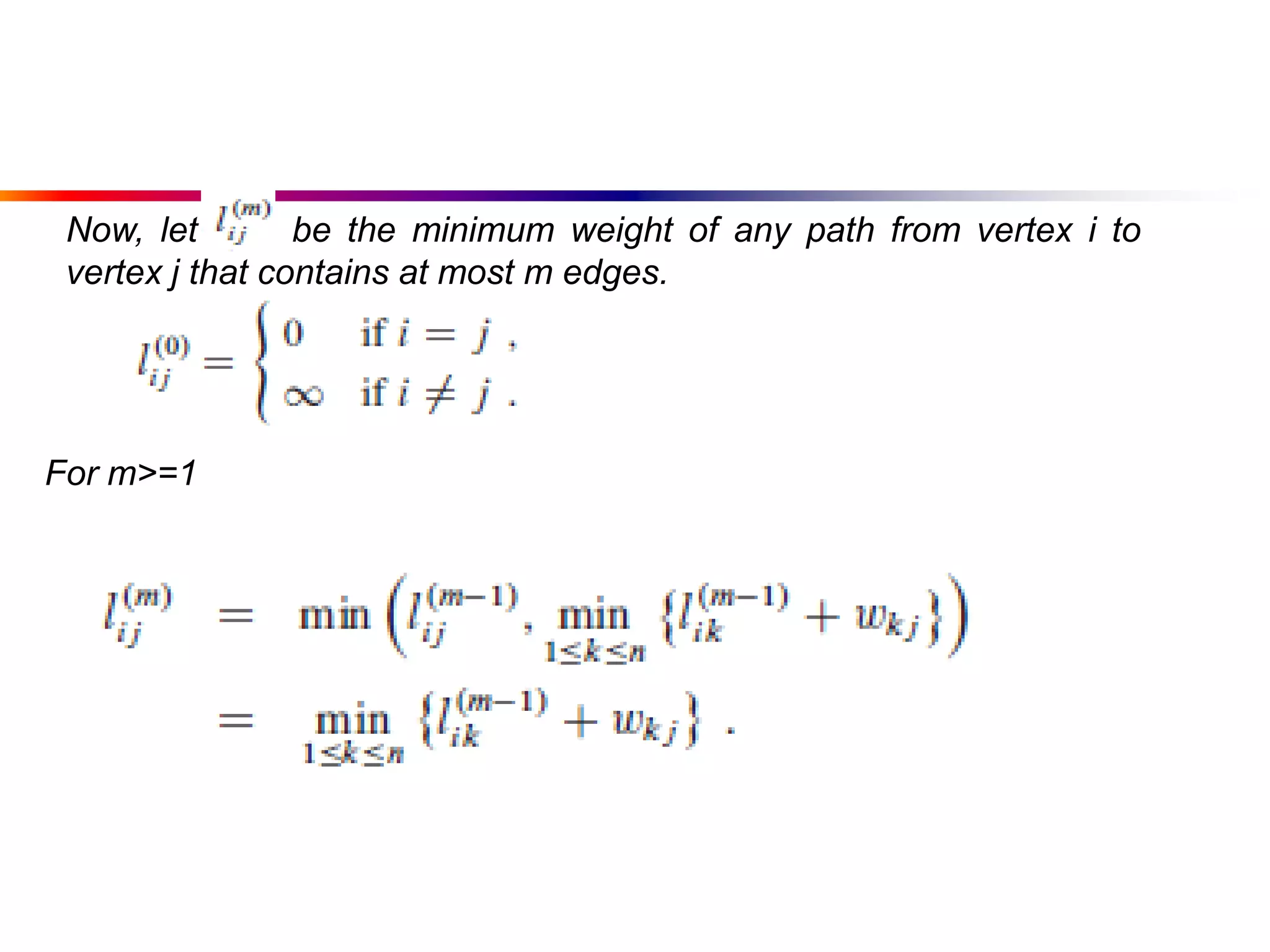
![Why Bellman-Ford Works
• On the first pass, we find d(s,u) for all vertices whose
shortest paths have one edge.
• On the second pass, the d[u] values computed for the one-
edge-away vertices are correct (= d(s,u)), so they are used
to compute the correct d values for vertices whose shortest
paths have two edges.
• Since no shortest path can have more than |V[G]|-1 edges,
after that many passes all d values are correct.
• Note: all vertices not reachable from s will have their
original values of infinity. (Same, by the way, for
Dijkstra).](https://image.slidesharecdn.com/lecture17-140420071825-phpapp02/75/Shortest-Path-in-Graph-27-2048.jpg)
![Bellman-Ford: Algorithm
● BELLMAN-FORD(G, w, s)
● 1 foreach vertex v V[G] do //INIT_SINGLE_SOURCE
● 2 d[v]
● 3 p[v] NIL
● 4 d[s] 0
● 5 for i 1 to |V[G]|-1 do > each iteration is a “pass”
● 6 for each edge (u,v) in E[G] do
● 7 RELAX(u, v, w)
● 8 > check for negative cycles
● 9 for each edge (u,v) in E[G] do
● 10 if d[v] > d[u] + w(u,v) then
● 11 return FALSE
● 12 return TRUE
Running time:(VE)](https://image.slidesharecdn.com/lecture17-140420071825-phpapp02/75/Shortest-Path-in-Graph-28-2048.jpg)
![Negative Cycle Detection
● What if there is a negative-weight
cycle reachable from s?
● Assume: d[u] d[x]+4
● d[v] d[u]+5
● d[x] d[v]-10
● Adding:
● d[u]+d[v]+d[x] d[x]+d[u]+d[v]-1
● Because it’s a cycle, vertices on left are same as those on right.
Thus we get 0 -1; a contradiction.
So for at least one edge (u,v),
● d[v] > d[u] + w(u,v)
● This is exactly what Bellman-Ford checks for.
u
x
v
4
5
-10](https://image.slidesharecdn.com/lecture17-140420071825-phpapp02/75/Shortest-Path-in-Graph-29-2048.jpg)


The document discusses algorithms for finding shortest paths in graphs. It describes Dijkstra's algorithm and Bellman-Ford algorithm for solving the single-source shortest paths problem and Floyd-Warshall algorithm for solving the all-pairs shortest paths problem. Dijkstra's algorithm uses a priority queue to efficiently find shortest paths from a single source node to all others, assuming non-negative edge weights. Bellman-Ford handles graphs with negative edge weights but is slower. Floyd-Warshall finds shortest paths between all pairs of nodes in a graph.
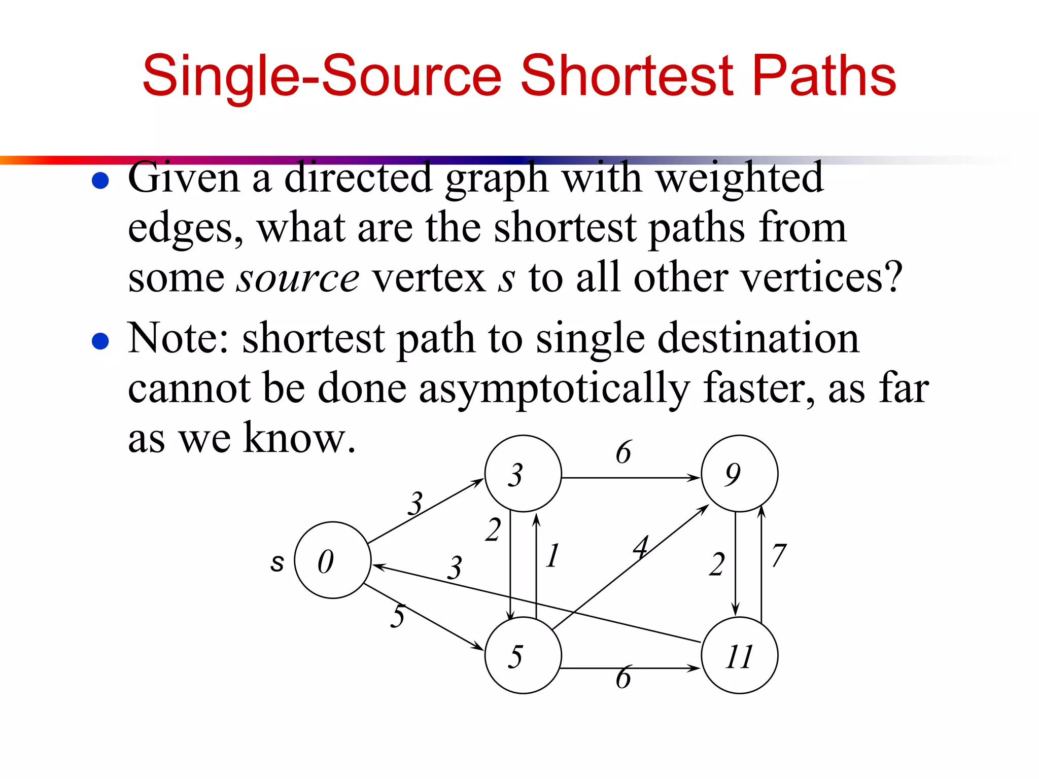
Introduction to shortest paths in directed graphs and the problems of finding single and all-pairs shortest paths.
Overview of various applications of shortest paths in graph algorithms.
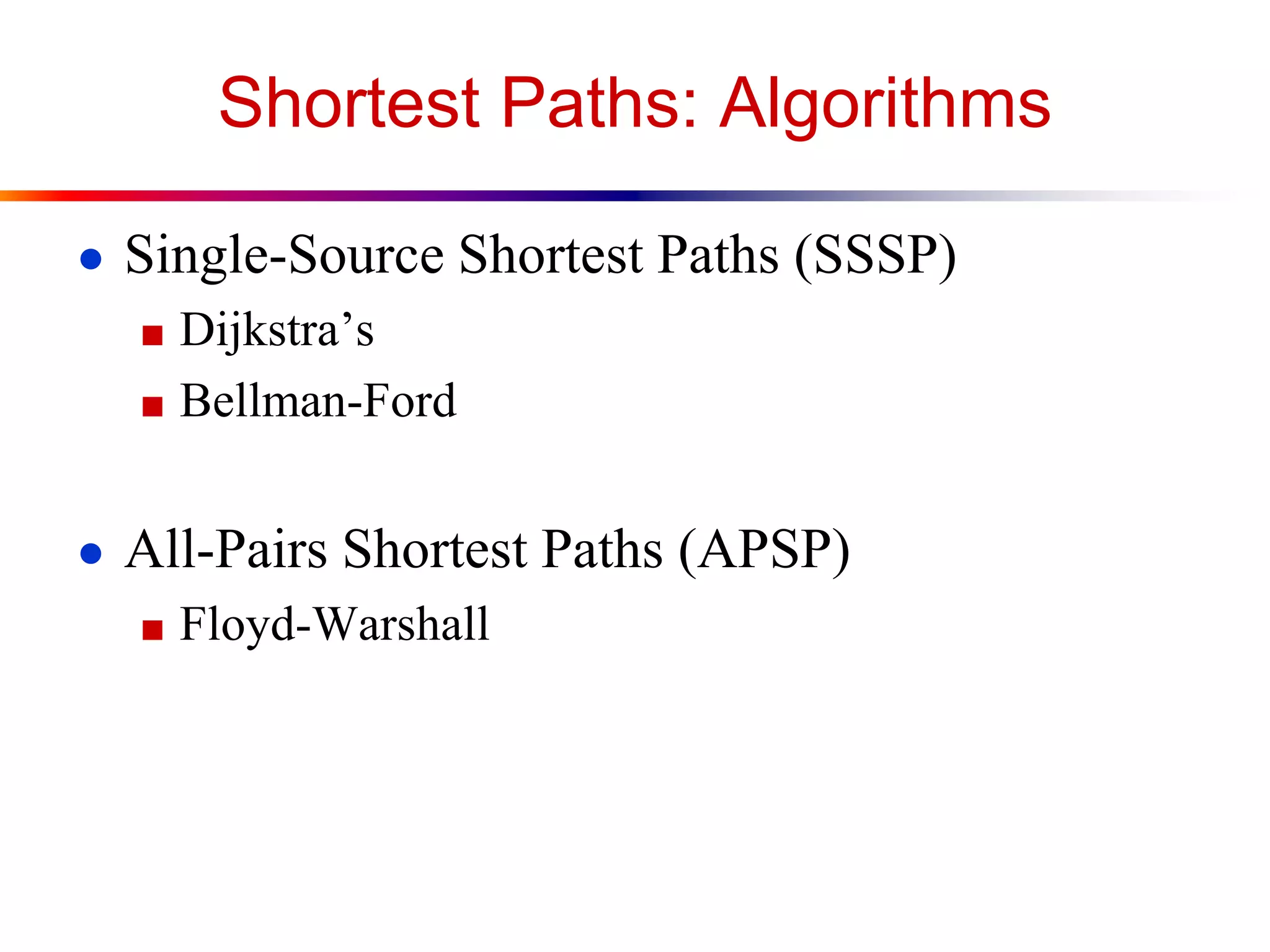
Introduction to algorithms for finding shortest paths: Dijkstra’s, Bellman-Ford for single-source and Floyd-Warshall for all-pairs.
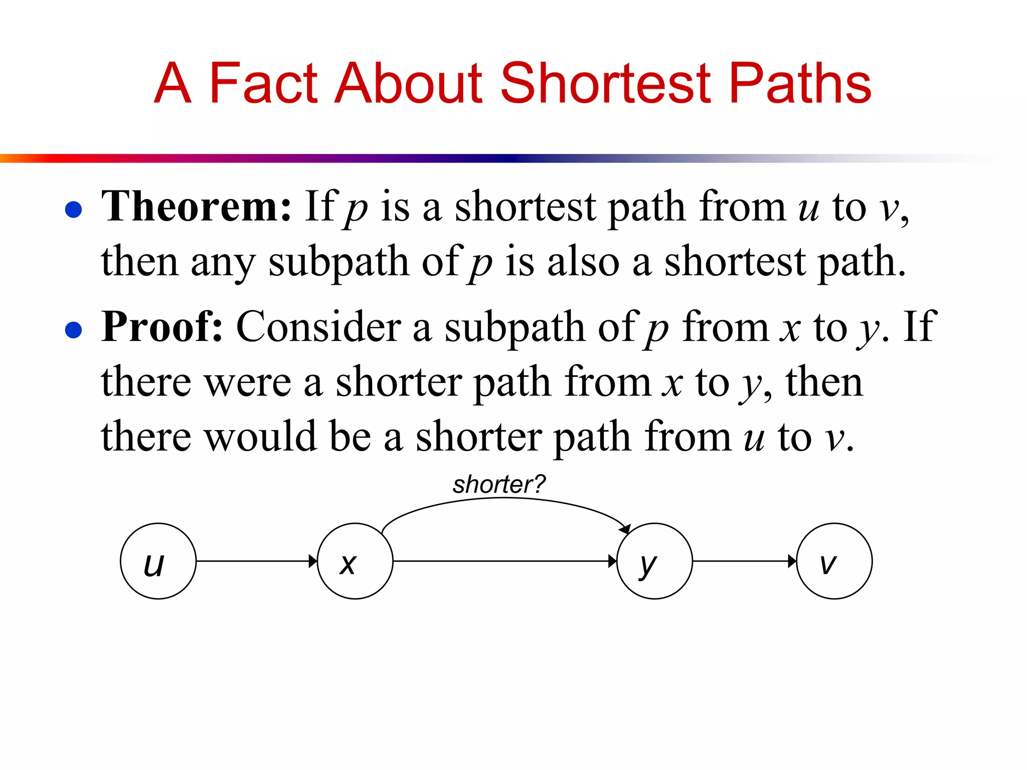
Theorem stating subpaths of shortest paths are also shortest paths, providing a fundamental property of shortest-path algorithms.
Details on SSSP, discussing the shortest paths from a source vertex to all others, and the updating mechanism for path lengths.
The RELAX operation that updates estimates of shortest paths and maintains the predecessor information during the algorithm.
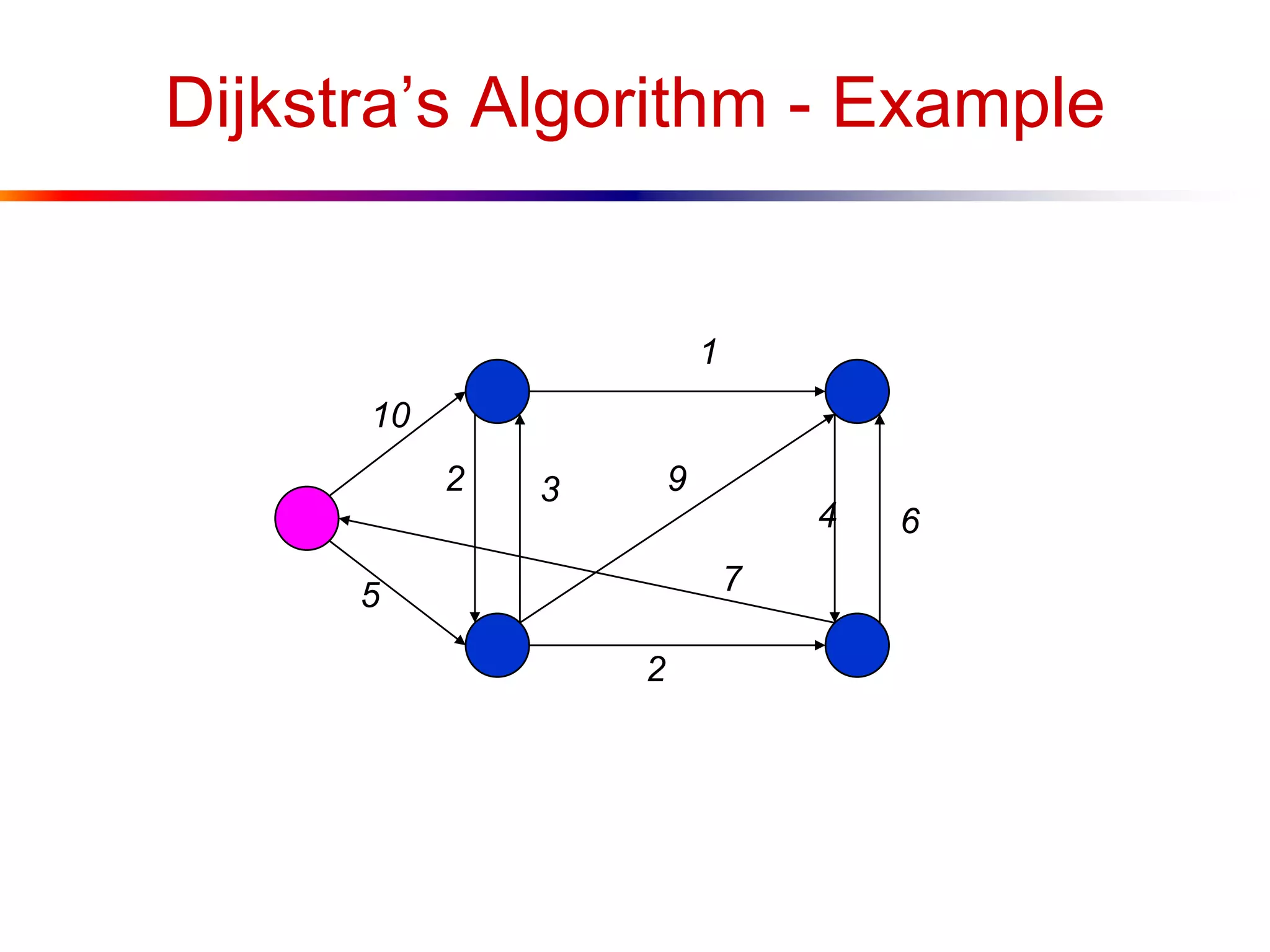
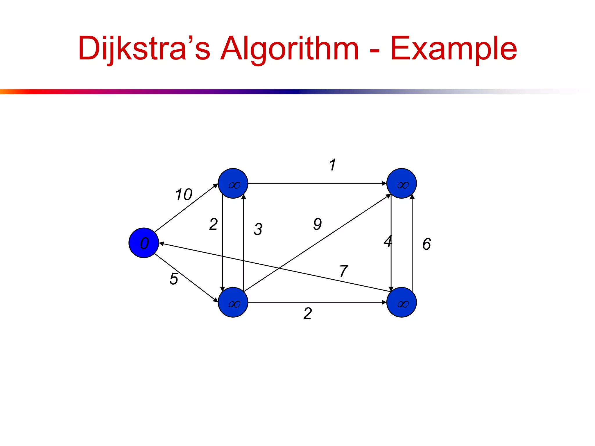
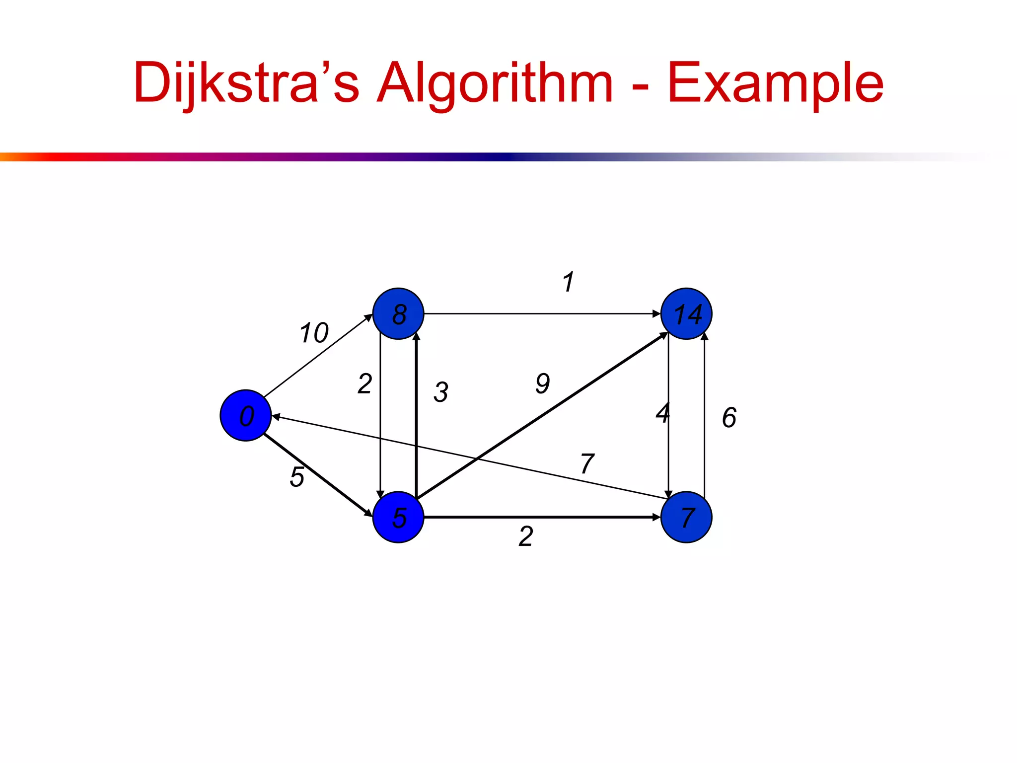
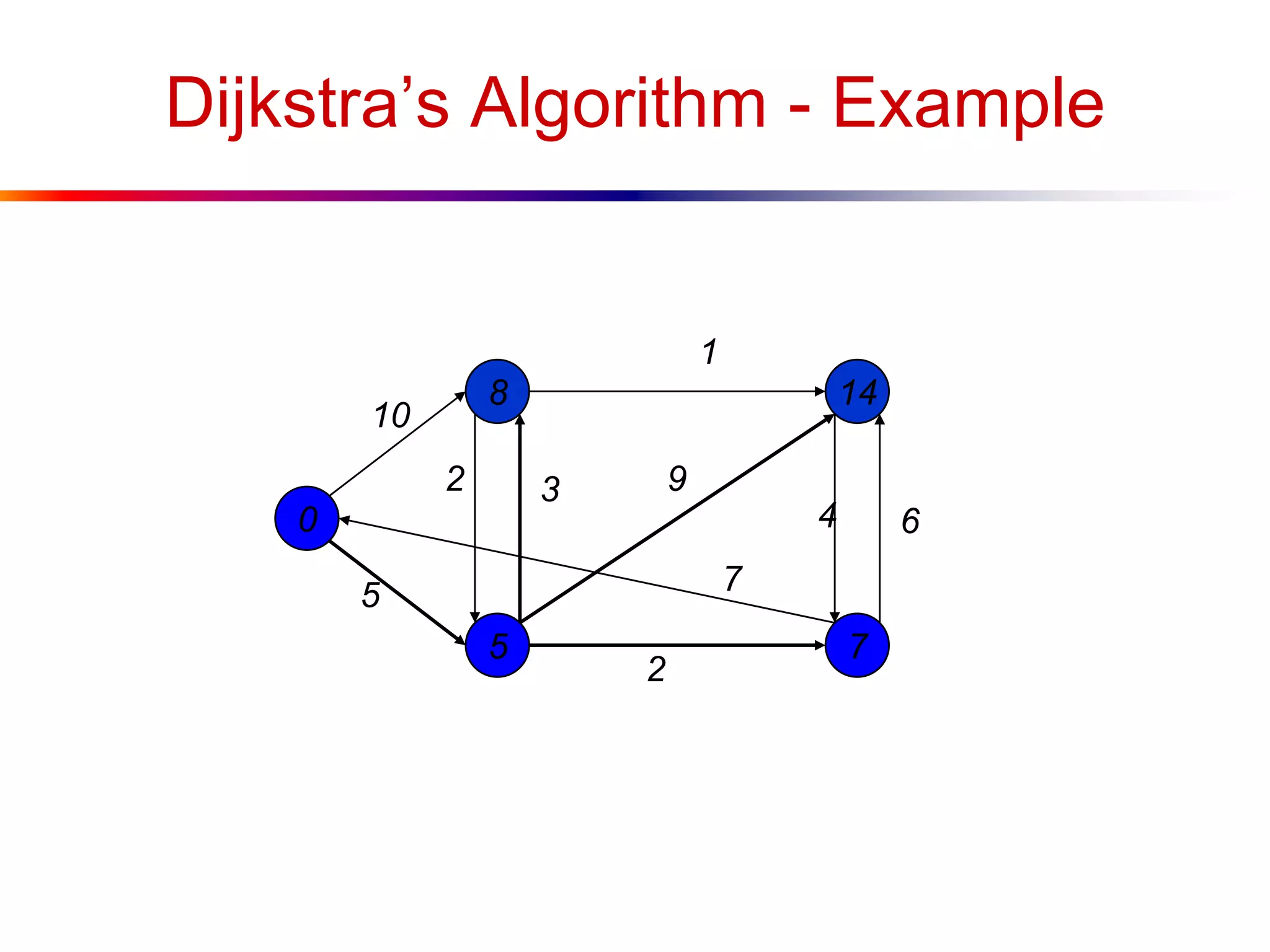
Introduction to Dijkstra's algorithm, assumptions of edge weights, and an overview of its working mechanism.
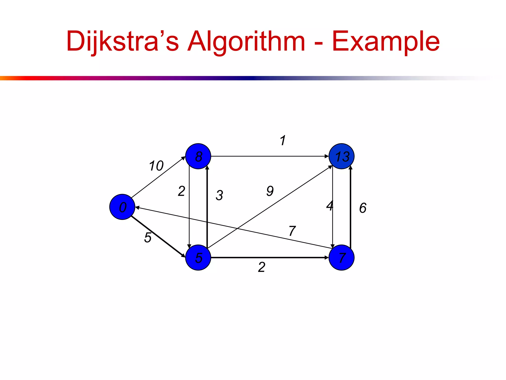
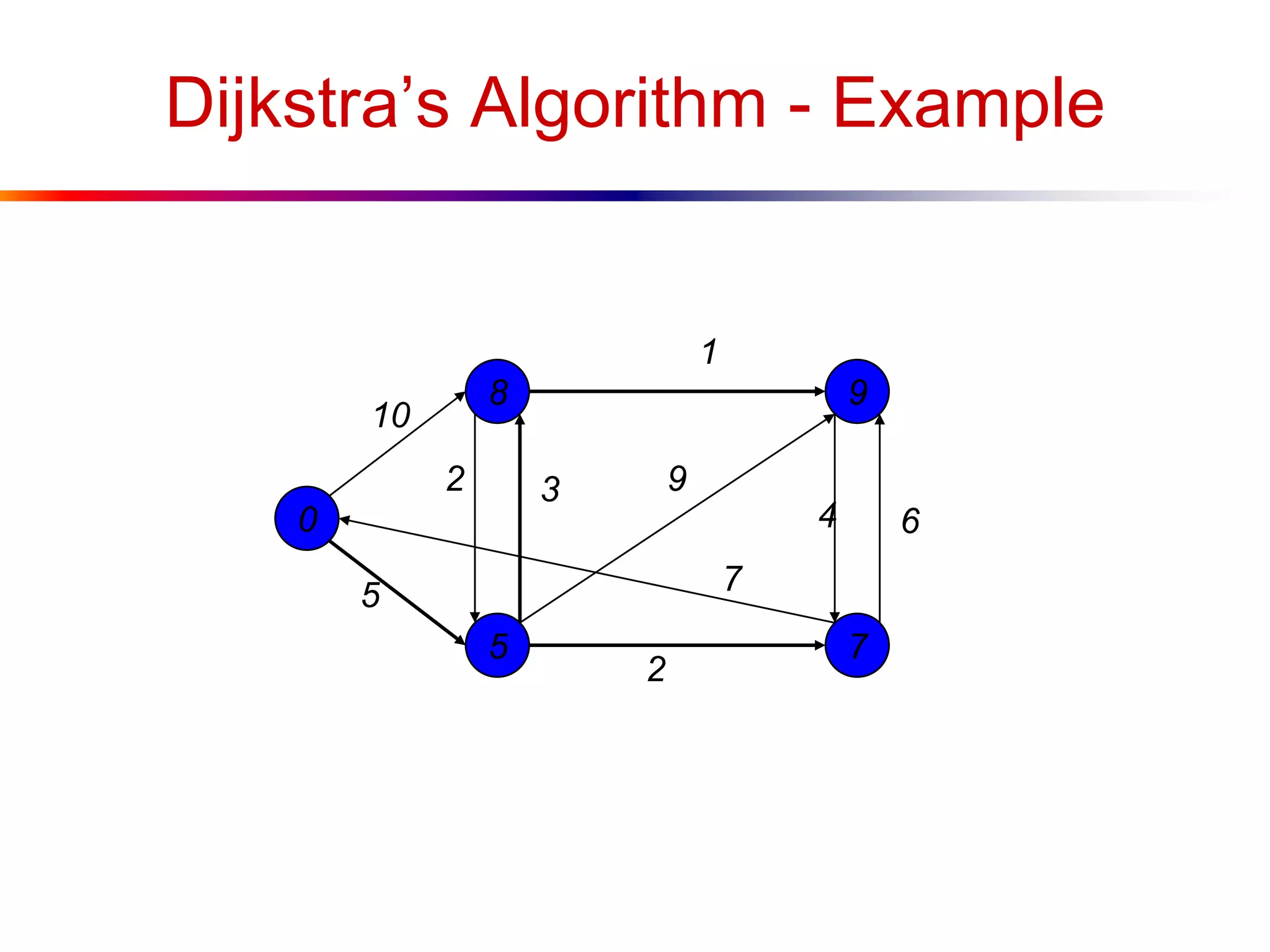
Detailed examples with matrices showing state changes at each step of Dijkstra's algorithm throughout the execution.
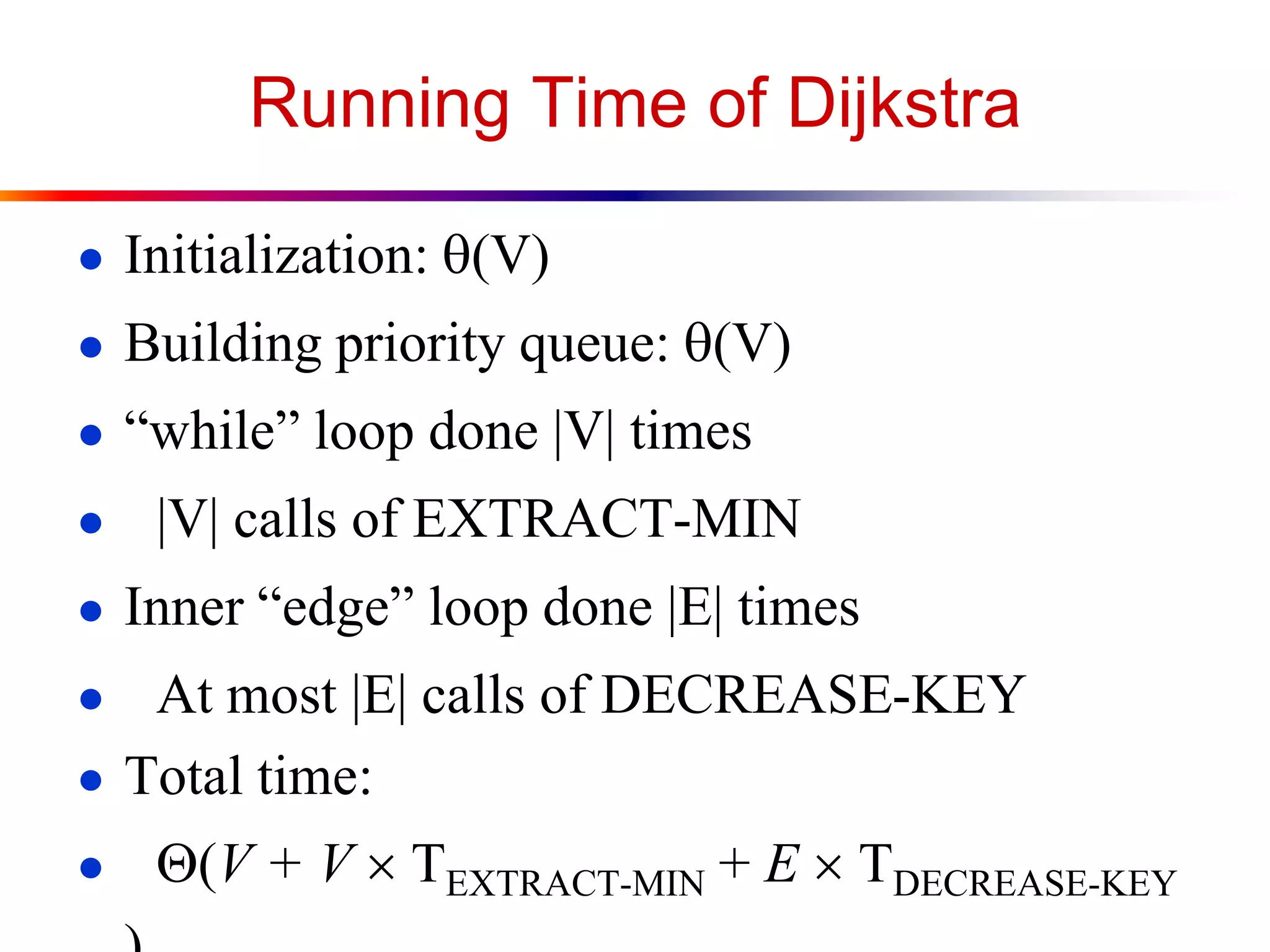
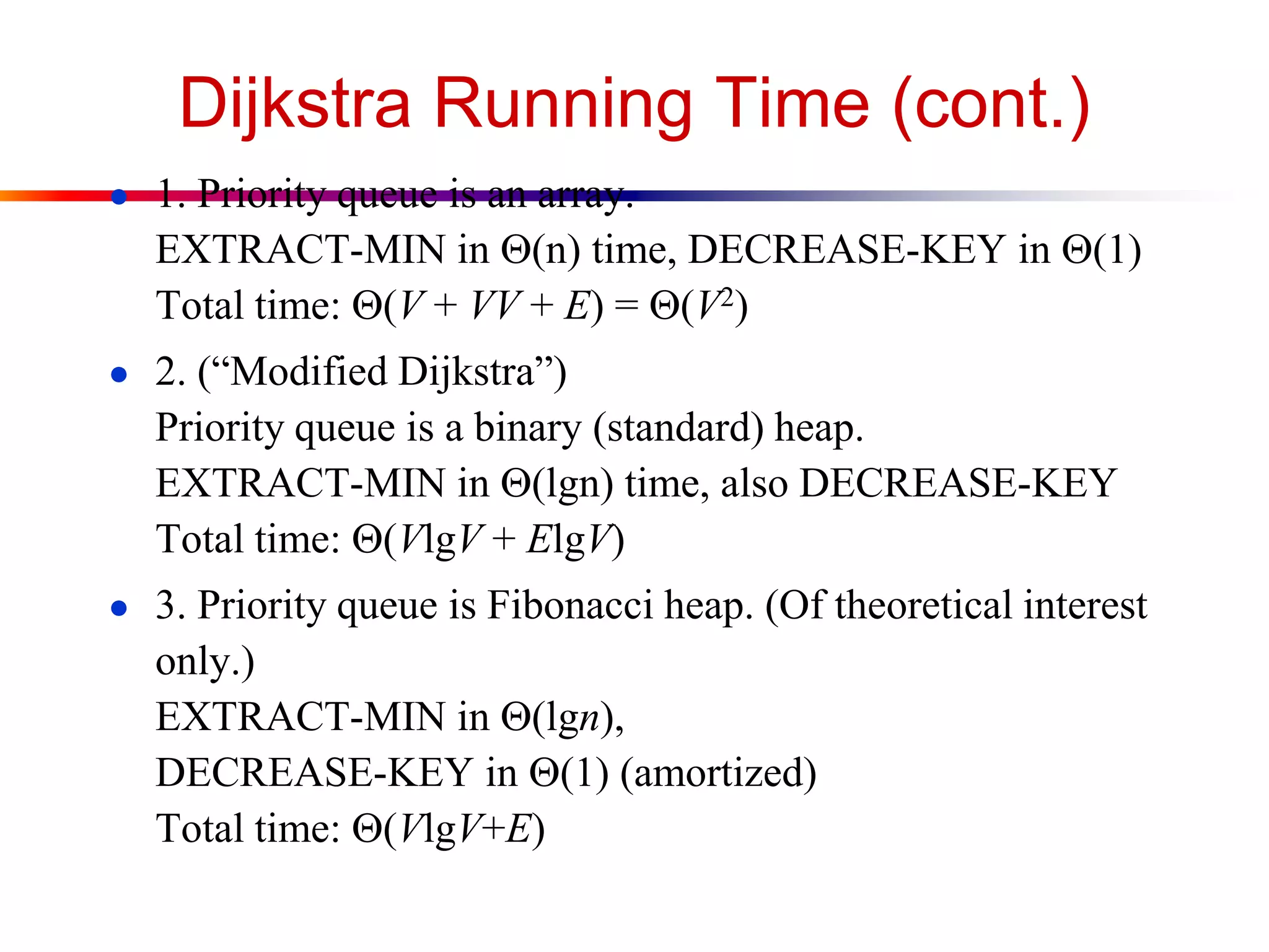
Discussion on the time complexity of Dijkstra's algorithm based on different priority queue implementations.
Overview of the Bellman-Ford algorithm, its capability to handle negative edge weights, and cycle detection.
Explanation of the Bellman-Ford algorithm's iterative relaxation method and running time analysis.
Demonstration of how Bellman-Ford detects negative cycles through contradictions based on shortest paths.
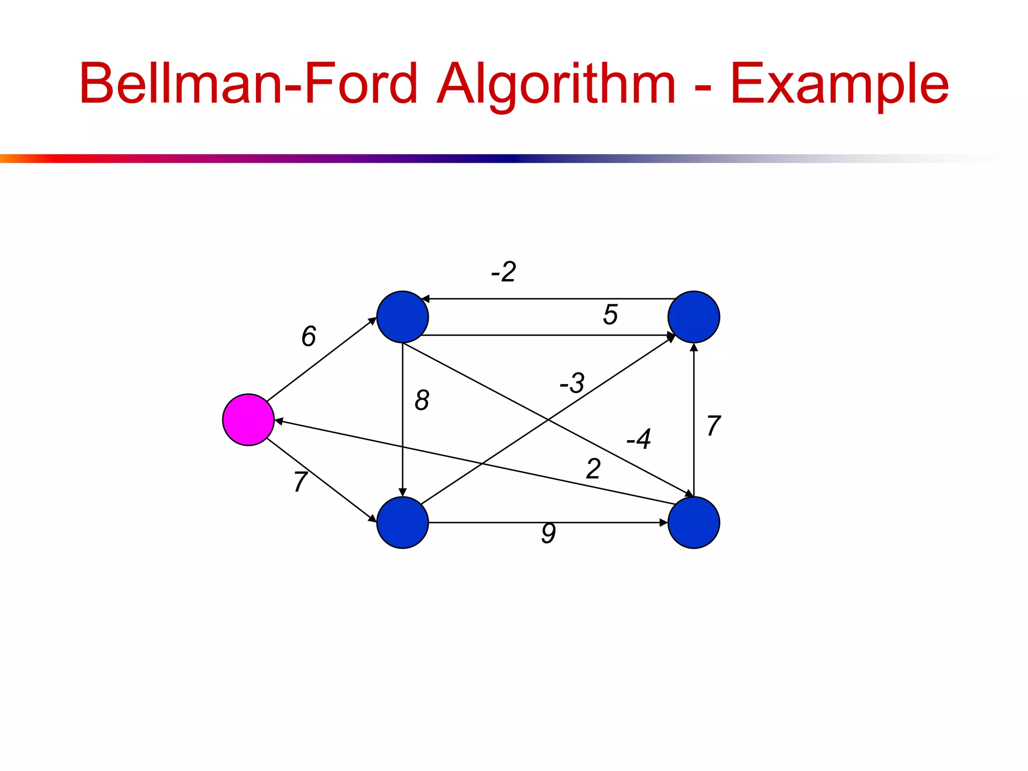
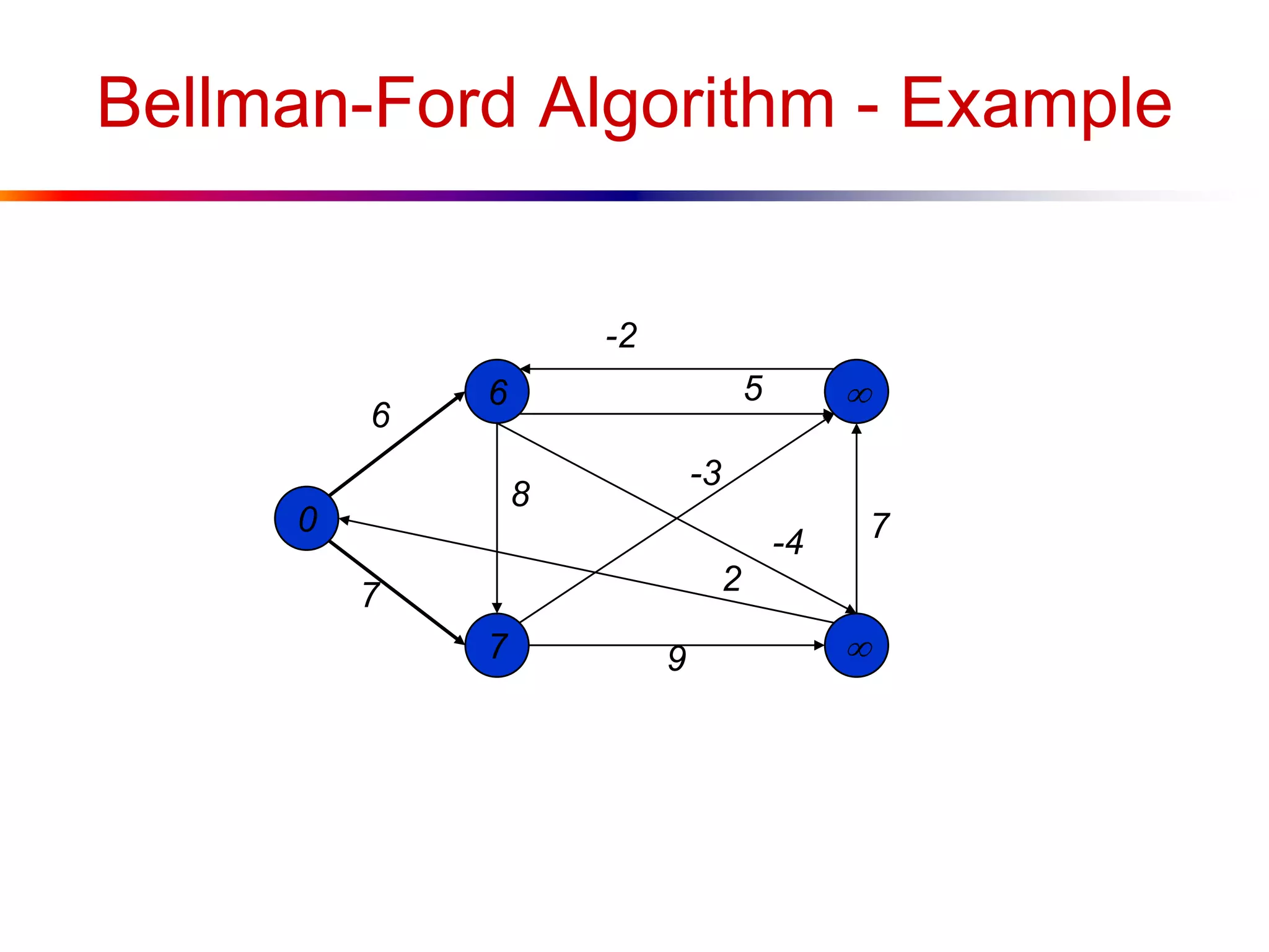
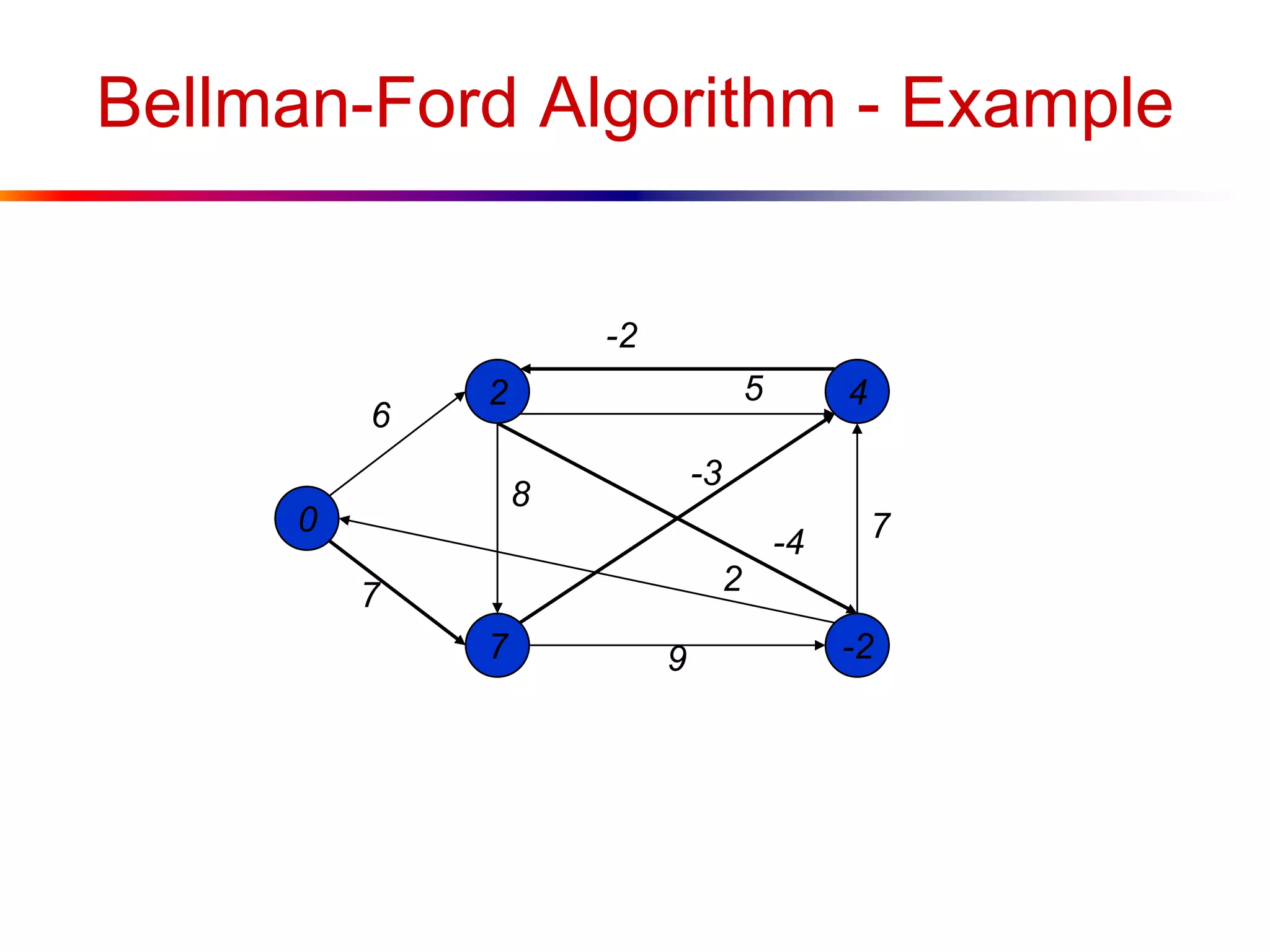
Step-by-step example of the Bellman-Ford algorithm and its execution results through a series of updates.
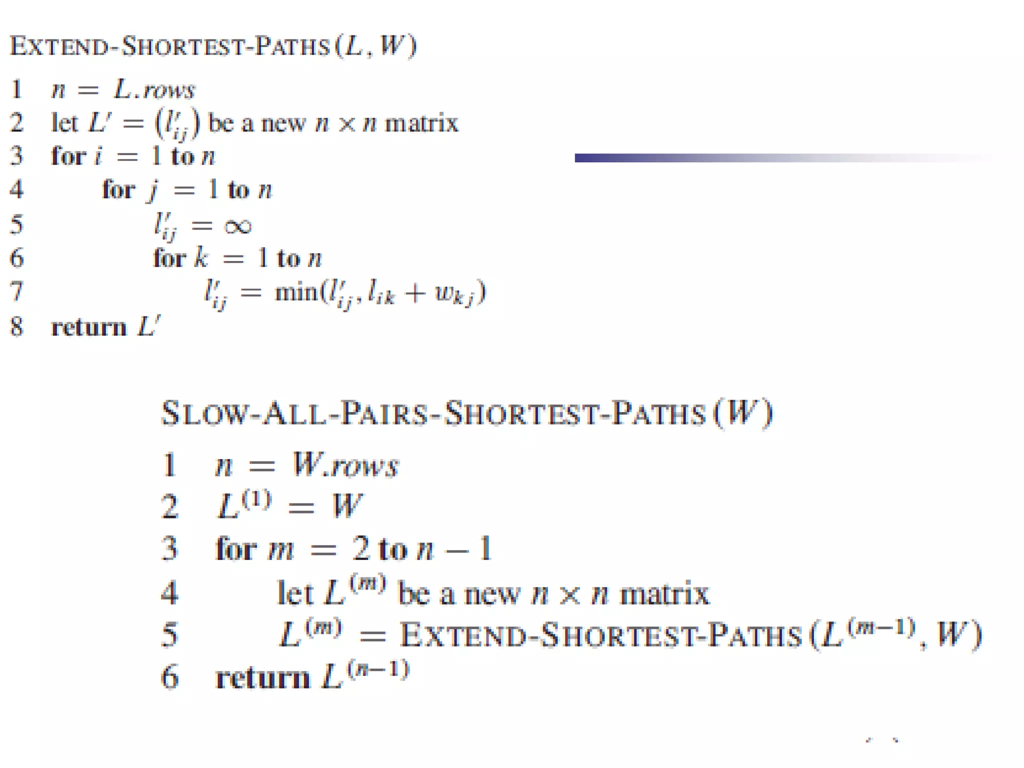
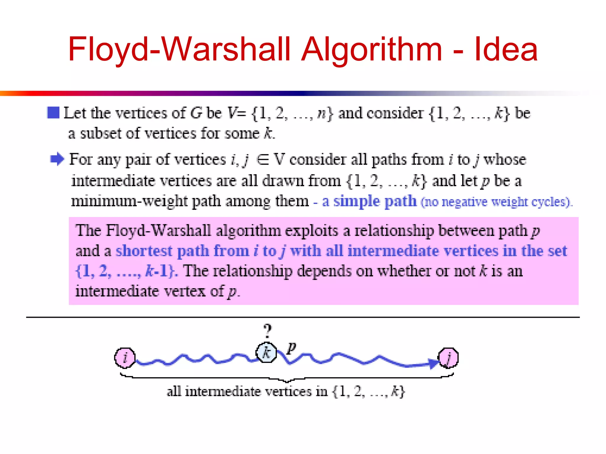
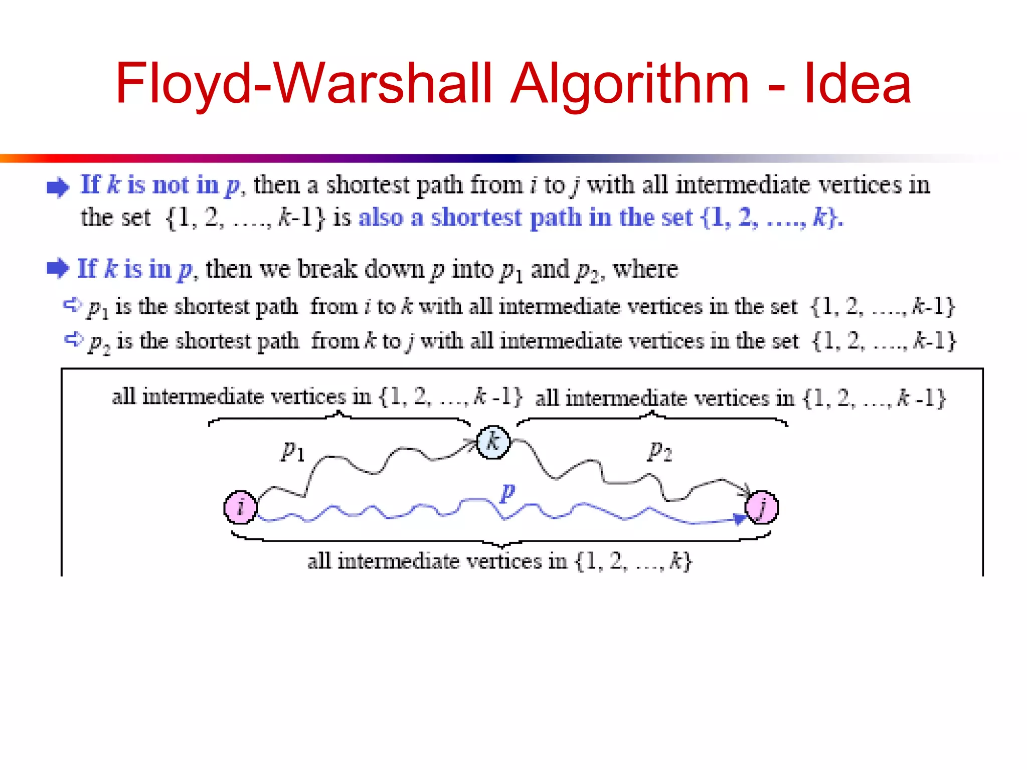
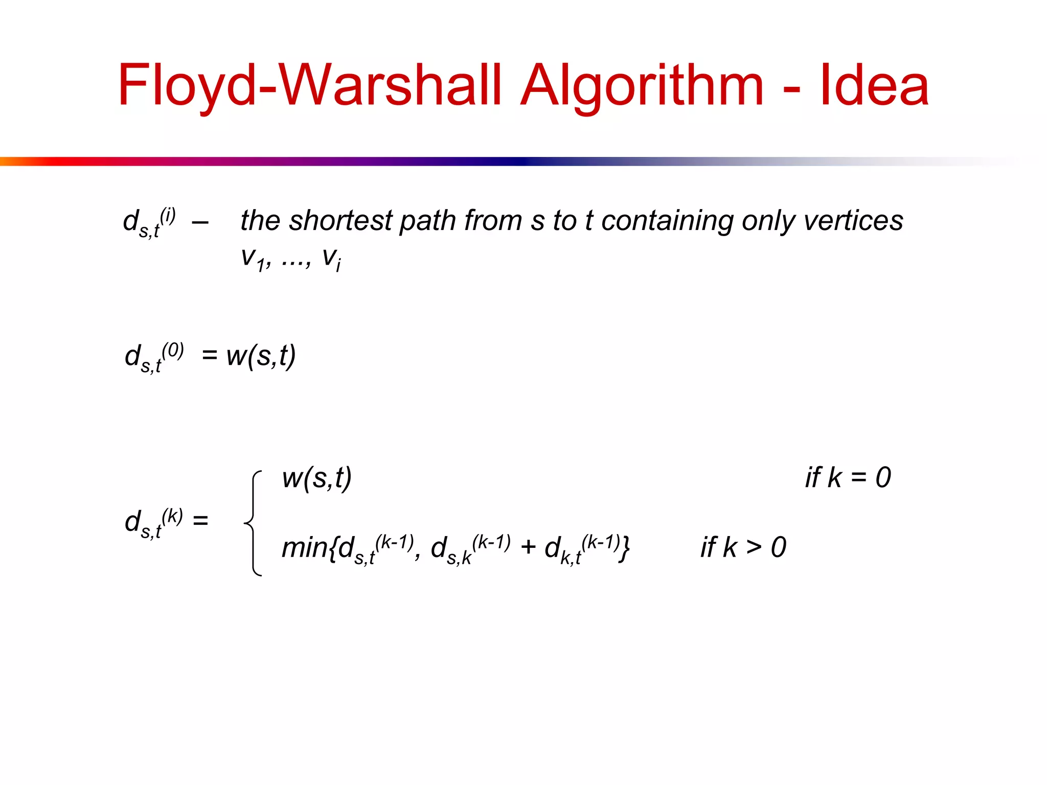
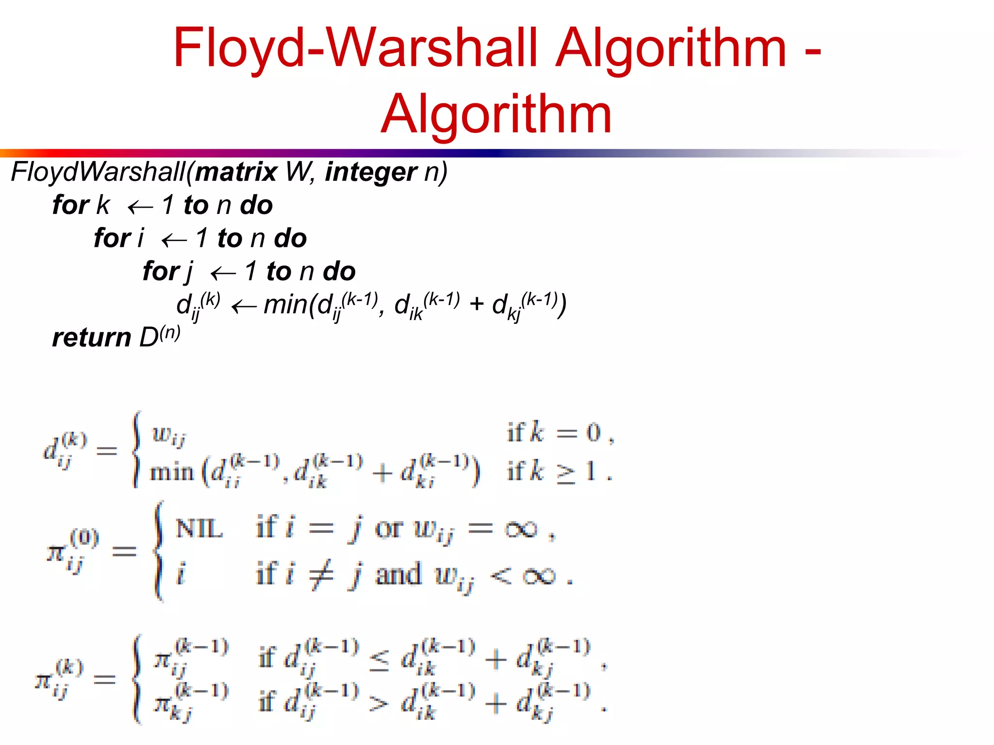
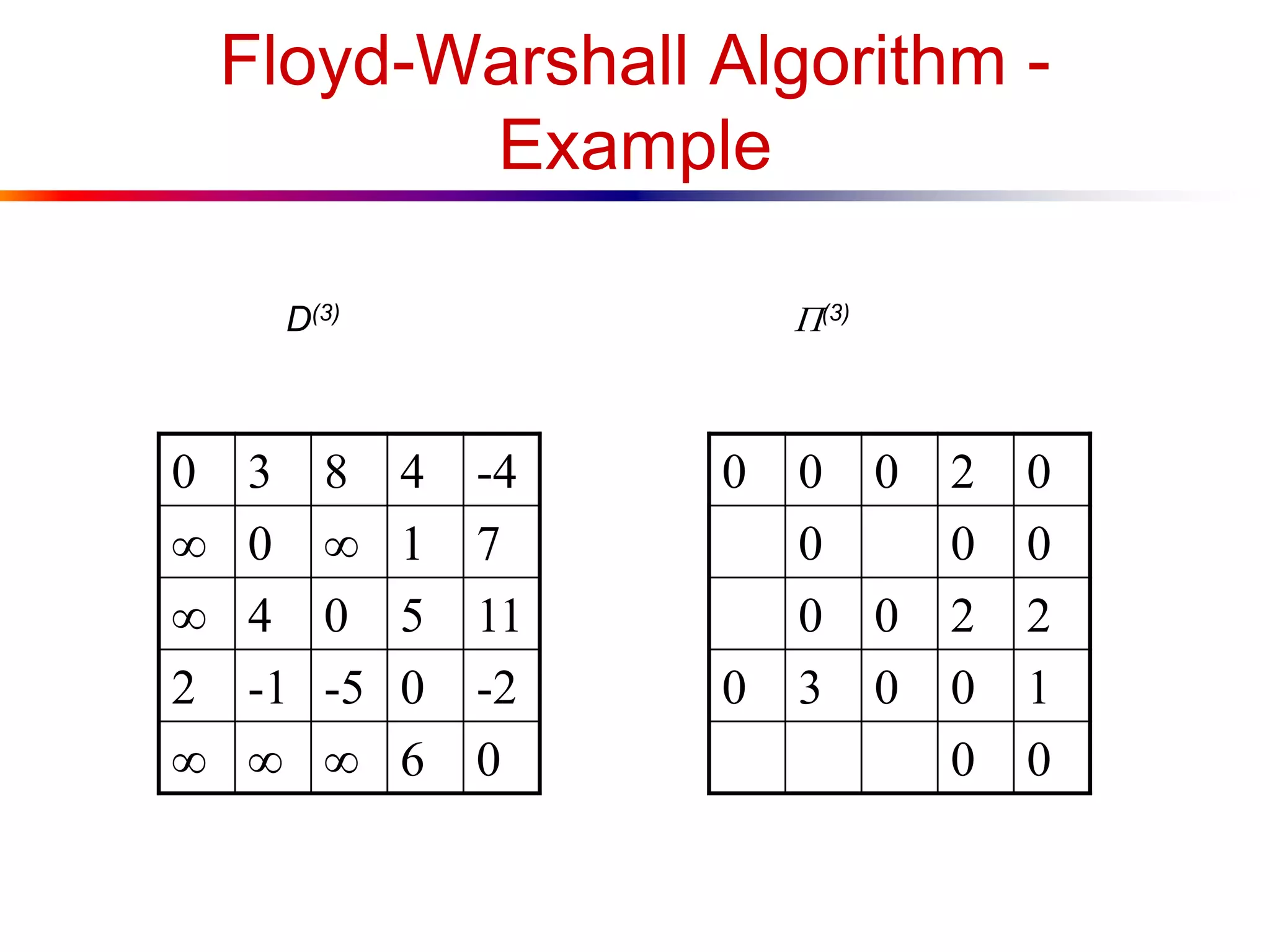
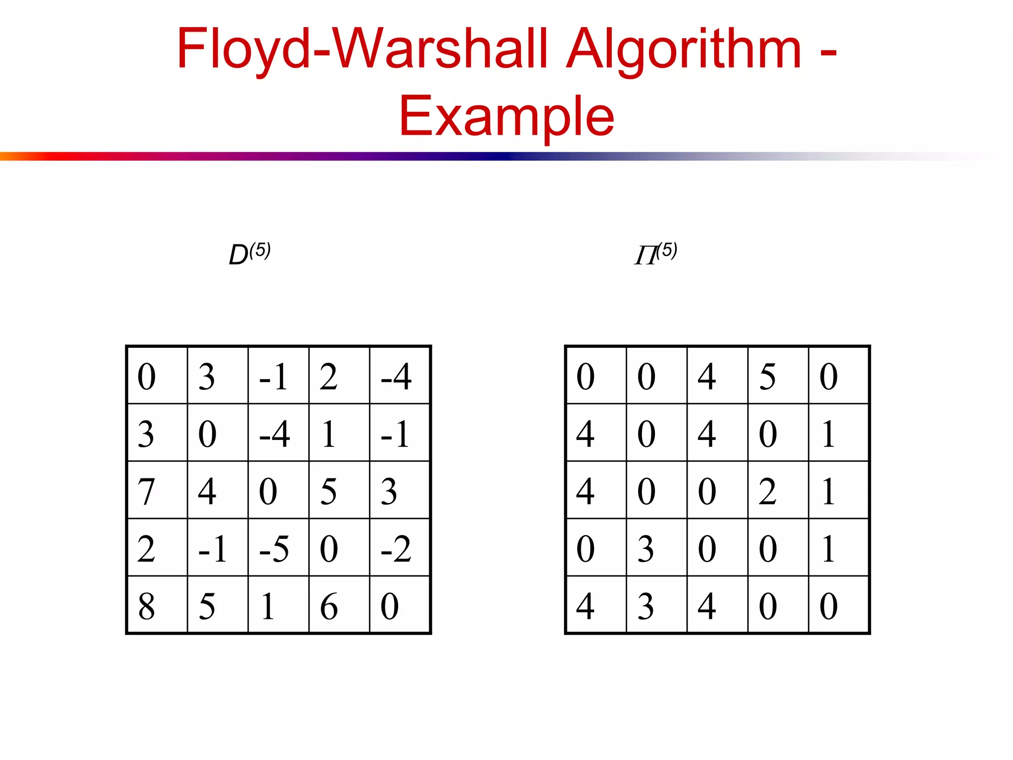
Introduction to the Floyd-Warshall algorithm’s idea, focusing on dynamic programming principles.
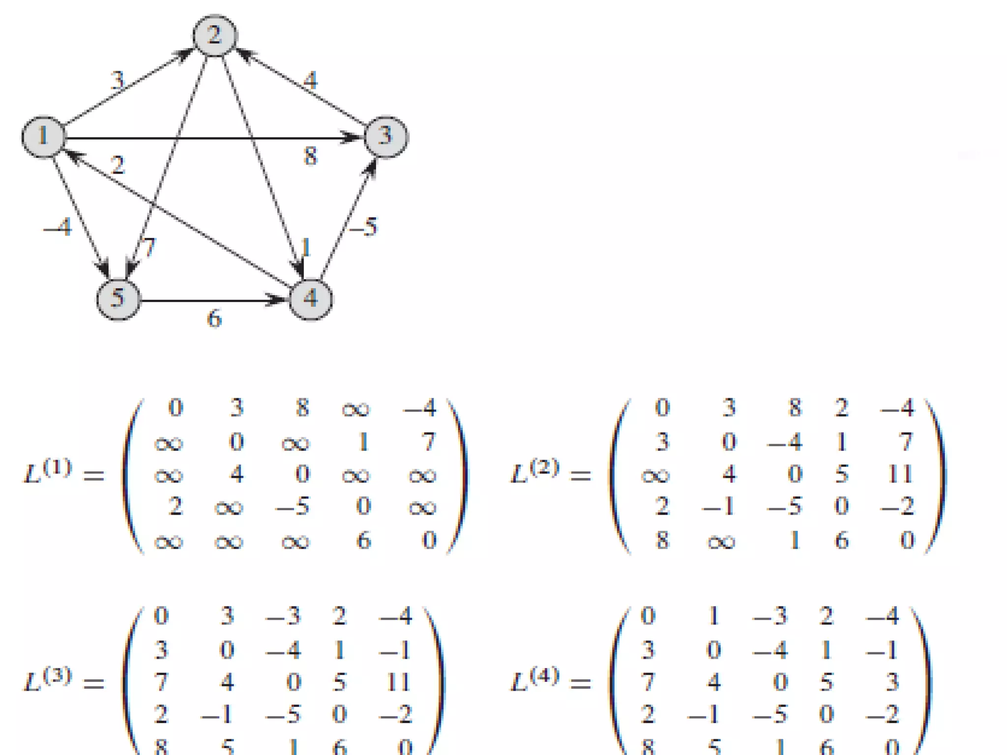
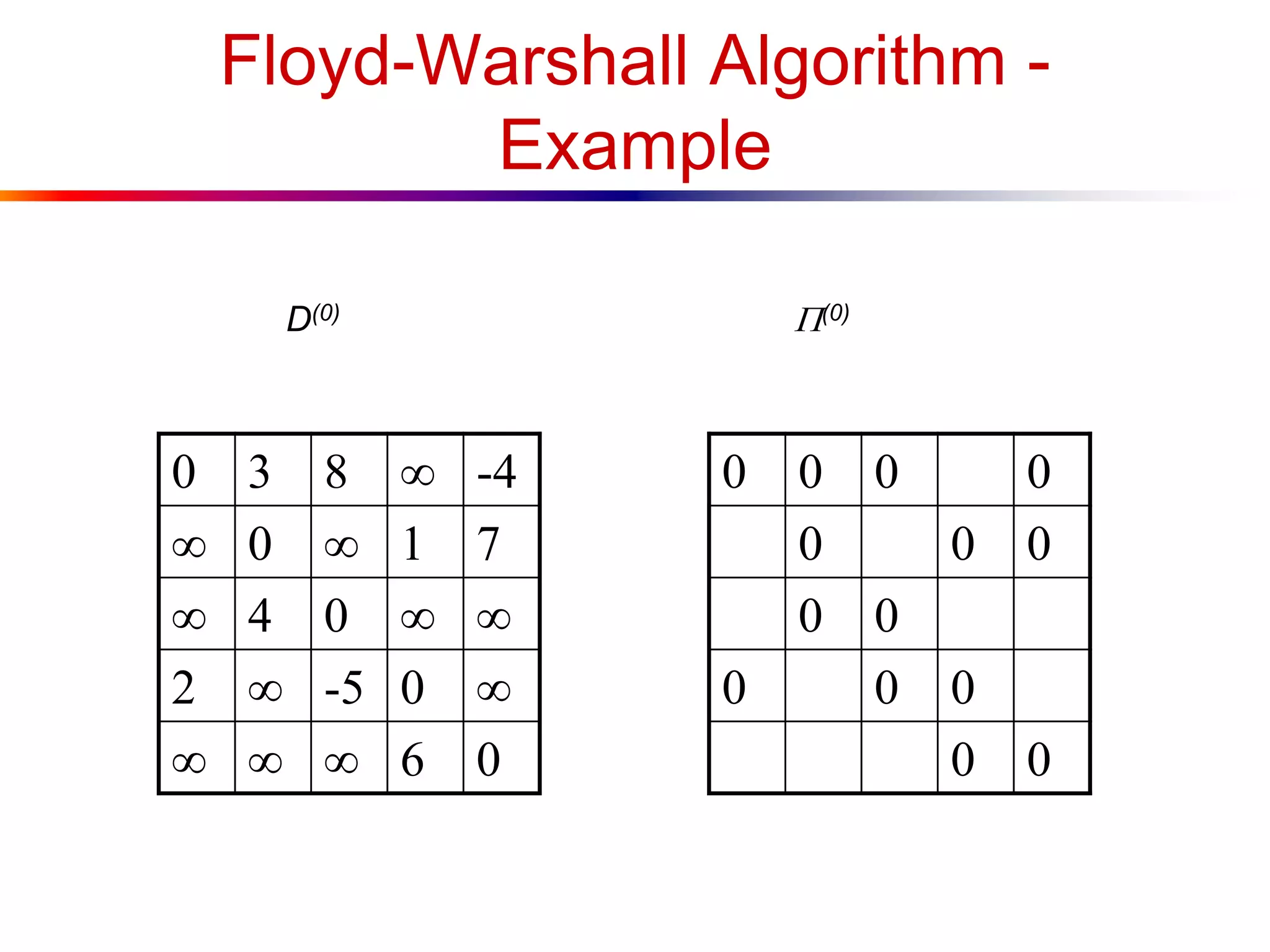
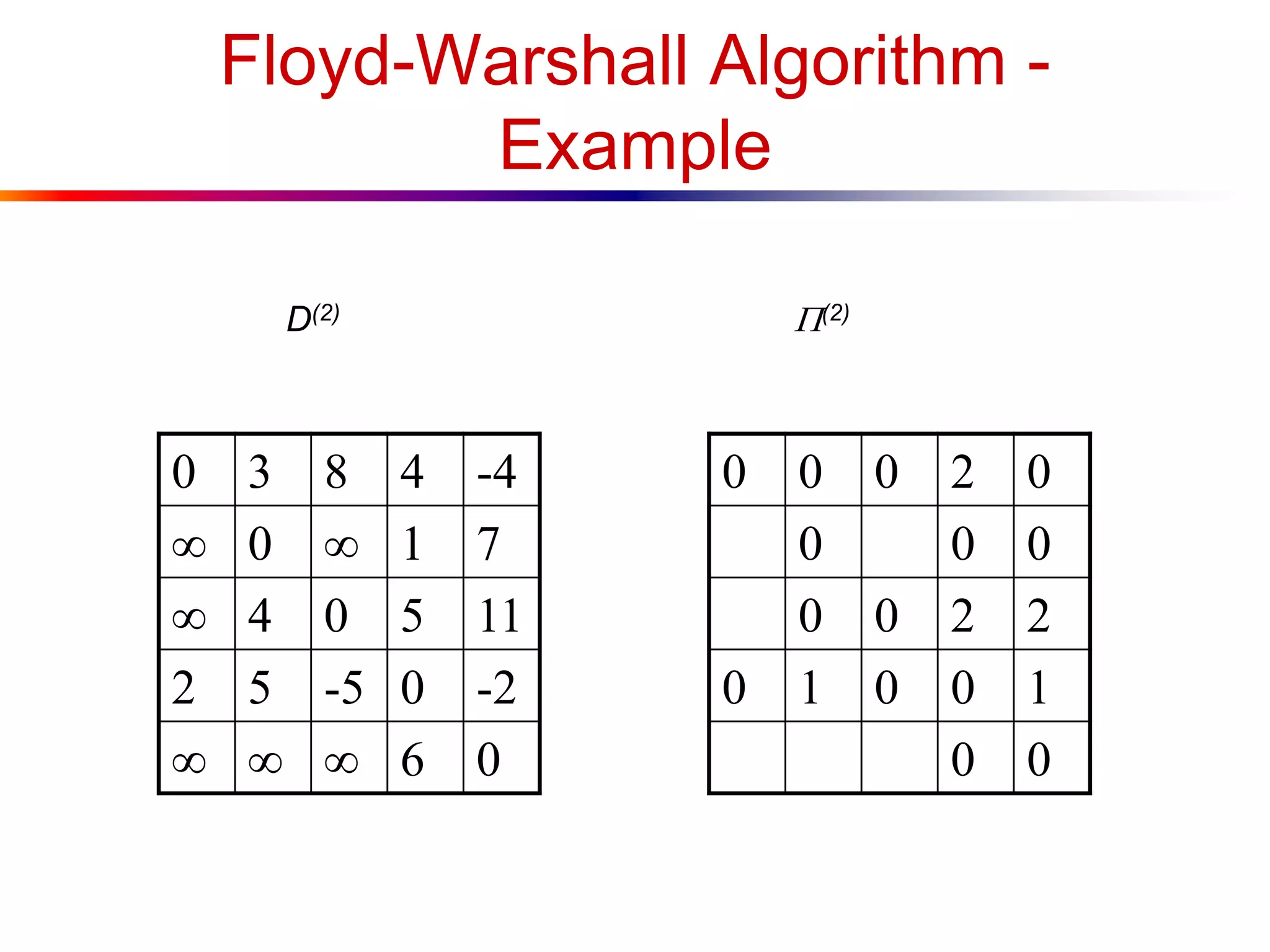
The detailed execution and series of examples demonstrating the Floyd-Warshall algorithm’s processing through matrices.