Analysis and Design of Algorithm
B. Tech. (CSE), VII Semester
Roshan Tailor
Amity University Rajasthan
2
This Lecture
• Single-source shortest paths in weighted graphs
– Shortest-Path Problems
– Properties of Shortest Paths, Relaxation
– Dijkstra’s Algorithm
– Bellman-Ford Algorithm
3
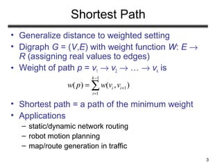
Shortest Path
• Generalize distance to weighted setting
• Digraph G = (V,E) with weight function W: E →
R (assigning real values to edges)
• Weight of path p = v1 → v2 → … → vk is
• Shortest path = a path of the minimum weight
• Applications
– static/dynamic network routing
– robot motion planning
– map/route generation in traffic
1
1
1
( ) ( , )
k
i i
i
w p w v v
−
+
=
= ∑
4
Shortest-Path Problems
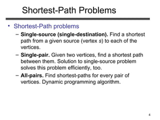
• Shortest-Path problems
– Single-source (single-destination). Find a shortest
path from a given source (vertex s) to each of the
vertices.
– Single-pair. Given two vertices, find a shortest path
between them. Solution to single-source problem
solves this problem efficiently, too.
– All-pairs. Find shortest-paths for every pair of
vertices. Dynamic programming algorithm.
5
Negative Weights and Cycles?
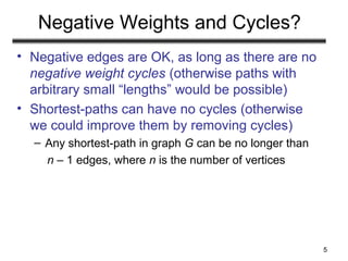
• Negative edges are OK, as long as there are no
negative weight cycles (otherwise paths with
arbitrary small “lengths” would be possible)
• Shortest-paths can have no cycles (otherwise
we could improve them by removing cycles)
– Any shortest-path in graph G can be no longer than
n – 1 edges, where n is the number of vertices
6
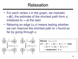
Relaxation
• For each vertex v in the graph, we maintain
v.d(), the estimate of the shortest path from s,
initialized to ∞ at the start
• Relaxing an edge (u,v) means testing whether
we can improve the shortest path to v found so
far by going through u
5
u v
vu
2
2
9
5 7
Relax(u,v)
5
u v
vu
2
2
6
5 6
Relax(u,v)
Relax (u,v,G)
if v.d > u.d()+ w(u,v) then
v.d = (u.d()+ w(u,v))
v.setparent = u
7
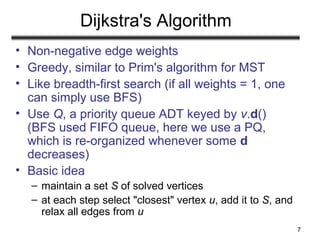
Dijkstra's Algorithm
• Non-negative edge weights
• Greedy, similar to Prim's algorithm for MST
• Like breadth-first search (if all weights = 1, one
can simply use BFS)
• Use Q, a priority queue ADT keyed by v.d()
(BFS used FIFO queue, here we use a PQ,
which is re-organized whenever some d
decreases)
• Basic idea
– maintain a set S of solved vertices
– at each step select "closest" vertex u, add it to S, and
relax all edges from u
8
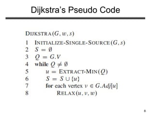
Dijkstra’s Pseudo Code
9
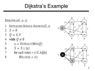
Dijkstra’s Example
∞ ∞
∞ ∞
0s
u v
yx
10
5
1
2 3
9
4 6
7
2
10 ∞
5 ∞
0s
u v
yx
10
5
1
2 3
9
4 6
7
2
10
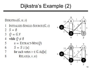
Dijkstra’s Example (2)
u v
8 14
5 7
0s
yx
10
5
1
2 3
9
4 6
7
2
8 13
5 7
0s
u v
yx
10
5
1
2 3
9
4 6
7
2
11
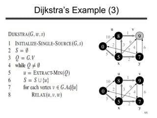
Dijkstra’s Example (3)
8 9
5 7
0
u v
yx
10
5
1
2 3
9
4 6
7
2
8 9
5 7
0
u v
yx
10
5
1
2 3
9
4 6
7
2
12
Dijkstra’s Running Time
• Extract-Min executed |V| time
• Decrease-Key executed |E| time
• Time = |V| TExtract-Min + |E| TDecrease-Key
• T depends on different Q implementations
Q T(Extract-
Min)
T(Decrease-Key) Total
array Ο(V) Ο(1) Ο(V 2
)
binary heap Ο(lg V) Ο(lg V) Ο(E lg V)
Fibonacci heap Ο(lg V) Ο(1) (amort.) Ο(V lgV + E)
13
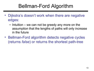
Bellman-Ford Algorithm
• Dijkstra’s doesn’t work when there are negative
edges:
– Intuition – we can not be greedy any more on the
assumption that the lengths of paths will only increase
in the future
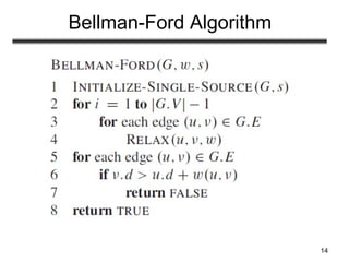
• Bellman-Ford algorithm detects negative cycles
(returns false) or returns the shortest path-tree
14
Bellman-Ford Algorithm
15
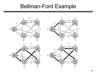
Bellman-Ford Example
5
∞ ∞
∞ ∞
0s
zy
6
7
8
-3
7
2
9
-2
xt
-4
6 ∞
7 ∞
0s
zy
6
7
8
-3
7
2
9
-2
xt
-4
5
6 4
7 2
0s
zy
6
7
8
-3
7
2
9
-2
xt
-4
5
2 4
7 2
0s
zy
6
7
8
-3
7
2
9
-2
xt
-4
5
16
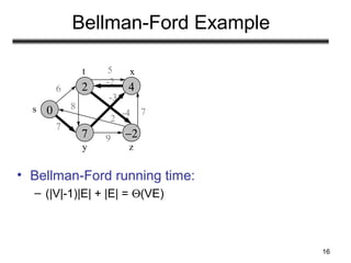
Bellman-Ford Example
2 4
7 −2
0s
zy
6
7
8
-3
7
2
9
-2
xt
-4
• Bellman-Ford running time:
– (|V|-1)|E| + |E| = Θ(VE)
5
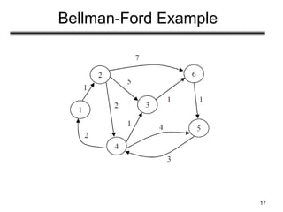
Bellman-Ford Example
17

Single source stortest path bellman ford and dijkstra

  • 1.
    Analysis and Designof Algorithm B. Tech. (CSE), VII Semester Roshan Tailor Amity University Rajasthan
  • 2.
    2 This Lecture • Single-sourceshortest paths in weighted graphs – Shortest-Path Problems – Properties of Shortest Paths, Relaxation – Dijkstra’s Algorithm – Bellman-Ford Algorithm
  • 3.
    3 Shortest Path • Generalizedistance to weighted setting • Digraph G = (V,E) with weight function W: E → R (assigning real values to edges) • Weight of path p = v1 → v2 → … → vk is • Shortest path = a path of the minimum weight • Applications – static/dynamic network routing – robot motion planning – map/route generation in traffic 1 1 1 ( ) ( , ) k i i i w p w v v − + = = ∑
  • 4.
    4 Shortest-Path Problems • Shortest-Pathproblems – Single-source (single-destination). Find a shortest path from a given source (vertex s) to each of the vertices. – Single-pair. Given two vertices, find a shortest path between them. Solution to single-source problem solves this problem efficiently, too. – All-pairs. Find shortest-paths for every pair of vertices. Dynamic programming algorithm.
  • 5.
    5 Negative Weights andCycles? • Negative edges are OK, as long as there are no negative weight cycles (otherwise paths with arbitrary small “lengths” would be possible) • Shortest-paths can have no cycles (otherwise we could improve them by removing cycles) – Any shortest-path in graph G can be no longer than n – 1 edges, where n is the number of vertices
  • 6.
    6 Relaxation • For eachvertex v in the graph, we maintain v.d(), the estimate of the shortest path from s, initialized to ∞ at the start • Relaxing an edge (u,v) means testing whether we can improve the shortest path to v found so far by going through u 5 u v vu 2 2 9 5 7 Relax(u,v) 5 u v vu 2 2 6 5 6 Relax(u,v) Relax (u,v,G) if v.d > u.d()+ w(u,v) then v.d = (u.d()+ w(u,v)) v.setparent = u
  • 7.
    7 Dijkstra's Algorithm • Non-negativeedge weights • Greedy, similar to Prim's algorithm for MST • Like breadth-first search (if all weights = 1, one can simply use BFS) • Use Q, a priority queue ADT keyed by v.d() (BFS used FIFO queue, here we use a PQ, which is re-organized whenever some d decreases) • Basic idea – maintain a set S of solved vertices – at each step select "closest" vertex u, add it to S, and relax all edges from u
  • 8.
  • 9.
    9 Dijkstra’s Example ∞ ∞ ∞∞ 0s u v yx 10 5 1 2 3 9 4 6 7 2 10 ∞ 5 ∞ 0s u v yx 10 5 1 2 3 9 4 6 7 2
  • 10.
    10 Dijkstra’s Example (2) uv 8 14 5 7 0s yx 10 5 1 2 3 9 4 6 7 2 8 13 5 7 0s u v yx 10 5 1 2 3 9 4 6 7 2
  • 11.
    11 Dijkstra’s Example (3) 89 5 7 0 u v yx 10 5 1 2 3 9 4 6 7 2 8 9 5 7 0 u v yx 10 5 1 2 3 9 4 6 7 2
  • 12.
    12 Dijkstra’s Running Time •Extract-Min executed |V| time • Decrease-Key executed |E| time • Time = |V| TExtract-Min + |E| TDecrease-Key • T depends on different Q implementations Q T(Extract- Min) T(Decrease-Key) Total array Ο(V) Ο(1) Ο(V 2 ) binary heap Ο(lg V) Ο(lg V) Ο(E lg V) Fibonacci heap Ο(lg V) Ο(1) (amort.) Ο(V lgV + E)
  • 13.
    13 Bellman-Ford Algorithm • Dijkstra’sdoesn’t work when there are negative edges: – Intuition – we can not be greedy any more on the assumption that the lengths of paths will only increase in the future • Bellman-Ford algorithm detects negative cycles (returns false) or returns the shortest path-tree
  • 14.
  • 15.
    15 Bellman-Ford Example 5 ∞ ∞ ∞∞ 0s zy 6 7 8 -3 7 2 9 -2 xt -4 6 ∞ 7 ∞ 0s zy 6 7 8 -3 7 2 9 -2 xt -4 5 6 4 7 2 0s zy 6 7 8 -3 7 2 9 -2 xt -4 5 2 4 7 2 0s zy 6 7 8 -3 7 2 9 -2 xt -4 5
  • 16.
    16 Bellman-Ford Example 2 4 7−2 0s zy 6 7 8 -3 7 2 9 -2 xt -4 • Bellman-Ford running time: – (|V|-1)|E| + |E| = Θ(VE) 5
  • 17.