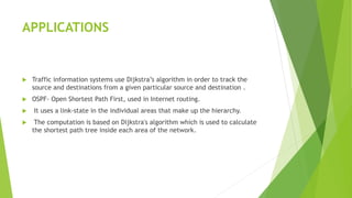
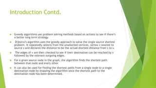
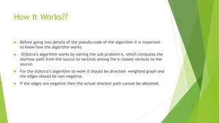
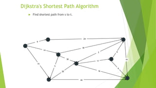
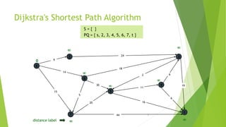
The document describes Dijkstra's algorithm for finding the shortest paths between nodes in a graph. It begins with an overview of how the algorithm works by solving subproblems to find the shortest path from the source to increasingly more nodes. It then provides pseudocode for the algorithm and analyzes its time complexity of O(E+V log V) when using a Fibonacci heap. Some applications of the algorithm include traffic information systems and routing protocols like OSPF.

1. SCHOOL MANAGEMENT SYSTEM
Submited BY:
Faisal Patel 254
Parth Bharuch 257
Dhavan Shah 160

2. Introduction
 Our project is about

3. Introduction Contd.
 Greedy algorithms use problem solving methods based on actions to see if there’s
a better long term strategy.
 Dijkstra’s algorithm uses the greedy approach to solve the single source shortest
problem. It repeatedly selects from the unselected vertices, vertex v nearest to
source s and declares the distance to be the actual shortest distance from s to v.
 The edges of v are then checked to see if their destination can be reached by v
followed by the relevant outgoing edges.
 For a given source node in the graph, the algorithm finds the shortest path
between that node and every other.
 It can also be used for finding the shortest paths from a single node to a single
destination node by stopping the algorithm once the shortest path to the
destination node has been determined.

4. How It Works??
 Before going into details of the pseudo-code of the algorithm it is important
to know how the algorithm works.
 Dijkstra’s algorithm works by solving the sub-problem k, which computes the
shortest path from the source to vertices among the k closest vertices to the
source.
 For the dijkstra’s algorithm to work it should be directed- weighted graph and
the edges should be non-negative.
 If the edges are negative then the actual shortest path cannot be obtained.

5. More Detailed Knowledge
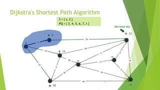
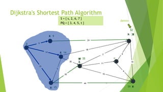
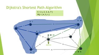
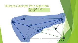
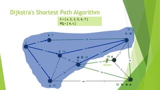
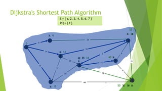
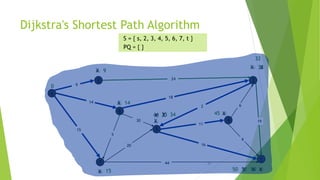
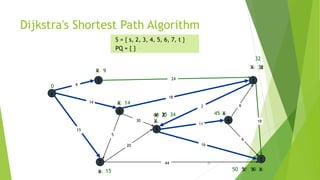
 At the kth round, there will be a set called Frontier of k vertices that will
consist of the vertices closest to the source and the vertices that lie outside
frontier are computed and put into New Frontier.
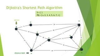
 The shortest distance obtained is maintained in sDist[w].
 It holds the estimate of the distance from s to w.
 Dijkstra’s algorithm finds the next closest vertex by maintaining the New
Frontier vertices in a priority-min queue.

6. 6
Dijkstra's Shortest Path Algorithm
 Find shortest path from s to t.
s
3
t
2
6
7
4
5
24
18
2
9
14
15
5
30
20
44
16
11
6
19
6

7. 7
Dijkstra's Shortest Path Algorithm
s
3
t
2
6
7
4
5
24
18
2
9
14
15
5
30
20
44
16
11
6
19
6







0
distance label
S = { }
PQ = { s, 2, 3, 4, 5, 6, 7, t }

8. 8
Dijkstra's Shortest Path Algorithm
s
3
t
2
6
7
4
5
24
18
2
9
14
15
5
30
20
44
16
11
6
19
6







0
distance label
S = { }
PQ = { s, 2, 3, 4, 5, 6, 7, t }
delmin

9. 9
Dijkstra's Shortest Path Algorithm
s
3
t
2
6
7
4
5
24
18
2
9
14
15
5
30
20
44
16
11
6
19
6
15
9



14

0
distance label
S = { s }
PQ = { 2, 3, 4, 5, 6, 7, t }
decrease key
X

X
X

10. 10
Dijkstra's Shortest Path Algorithm
s
3
t
2
6
7
4
5
24
18
2
9
14
15
5
30
20
44
16
11
6
19
6
15
9



14

0
distance label
S = { s }
PQ = { 2, 3, 4, 5, 6, 7, t }
X

X
X
delmin

11. 11
Dijkstra's Shortest Path Algorithm
s
3
t
2
6
7
4
5
24
18
2
9
14
15
5
30
20
44
16
11
6
19
6
15
9



14

0
S = { s, 2 }
PQ = { 3, 4, 5, 6, 7, t }
X

X
X

12. 12
Dijkstra's Shortest Path Algorithm
s
3
t
2
6
7
4
5
24
18
2
9
14
15
5
30
20
44
16
11
6
19
6
15
9



14

0
S = { s, 2 }
PQ = { 3, 4, 5, 6, 7, t }
X

X
X
decrease key
X 33

13. 13
Dijkstra's Shortest Path Algorithm
s
3
t
2
6
7
4
5
24
18
2
9
14
15
5
30
20
44
16
11
6
19
6
15
9



14

0
S = { s, 2 }
PQ = { 3, 4, 5, 6, 7, t }
X

X
X
X 33
delmin

14. 14
Dijkstra's Shortest Path Algorithm
s
3
t
2
6
7
4
5
24
18
2
9
14
15
5
30
20
44
16
11
6
19
6
15
9



14

0
S = { s, 2, 6 }
PQ = { 3, 4, 5, 7, t }
X

X
X
X 33
44
X
X
32

15. 15
Dijkstra's Shortest Path Algorithm
s
3
t
2
6
7
4
5
24
18
2
9
14
15
5
30
20
44
16
11
6
19
6
15
9


14

0
S = { s, 2, 6 }
PQ = { 3, 4, 5, 7, t }
X

X
X
44
X
delmin
X 33X
32

16. 16
Dijkstra's Shortest Path Algorithm
s
3
t
2
6
7
4
5
18
2
9
14
15
5
30
20
44
16
11
6
19
6
15
9


14

0
S = { s, 2, 6, 7 }
PQ = { 3, 4, 5, t }
X

X
X
44
X
35X
59 X
24
X 33X
32

17. 17
Dijkstra's Shortest Path Algorithm
s
3
t
2
6
7
4
5
24
18
2
9
14
15
5
30
20
44
16
11
6
19
6
15
9


14

0
S = { s, 2, 6, 7 }
PQ = { 3, 4, 5, t }
X

X
X
44
X
35X
59 X
delmin
X 33X
32

18. 18
Dijkstra's Shortest Path Algorithm
s
3
t
2
6
7
4
5
24
18
2
9
14
15
5
30
20
44
16
11
6
19
6
15
9


14

0
S = { s, 2, 3, 6, 7 }
PQ = { 4, 5, t }
X

X
X
44
X
35X
59 XX51
X 34
X 33X
32

19. 19
Dijkstra's Shortest Path Algorithm
s
3
t
2
6
7
4
5
18
2
9
14
15
5
30
20
44
16
11
6
19
6
15
9


14

0
S = { s, 2, 3, 6, 7 }
PQ = { 4, 5, t }
X

X
X
44
X
35X
59 XX51
X 34
delmin
X 33X
32
24

20. 20
Dijkstra's Shortest Path Algorithm
s
3
t
2
6
7
4
5
18
2
9
14
15
5
30
20
44
16
11
6
19
6
15
9


14

0
S = { s, 2, 3, 5, 6, 7 }
PQ = { 4, t }
X

X
X
44
X
35X
59 XX51
X 34
24
X50
X45
X 33X
32

21. 21
Dijkstra's Shortest Path Algorithm
s
3
t
2
6
7
4
5
18
2
9
14
15
5
30
20
44
16
11
6
19
6
15
9


14

0
S = { s, 2, 3, 5, 6, 7 }
PQ = { 4, t }
X

X
X
44
X
35X
59 XX51
X 34
24
X50
X45
delmin
X 33X
32

22. 22
Dijkstra's Shortest Path Algorithm
s
3
t
2
6
7
4
5
18
2
9
14
15
5
30
20
44
16
11
6
19
6
15
9


14

0
S = { s, 2, 3, 4, 5, 6, 7 }
PQ = { t }
X

X
X
44
X
35X
59 XX51
X 34
24
X50
X45
X 33X
32

23. 23
Dijkstra's Shortest Path Algorithm
s
3
t
2
6
7
4
5
18
2
9
14
15
5
30
20
44
16
11
6
19
6
15
9


14

0
S = { s, 2, 3, 4, 5, 6, 7 }
PQ = { t }
X

X
X
44
X
35X
59 XX51
X 34
X50
X45
delmin
X 33X
32
24

24. 24
Dijkstra's Shortest Path Algorithm
s
3
t
2
6
7
4
5
24
18
2
9
14
15
5
30
20
44
16
11
6
19
6
15
9


14

0
S = { s, 2, 3, 4, 5, 6, 7, t }
PQ = { }
X

X
X
44
X
35X
59 XX51
X 34
X50
X45
X 33X
32

25. 25
Dijkstra's Shortest Path Algorithm
s
3
t
2
6
7
4
5
24
18
2
9
14
15
5
30
20
44
16
11
6
19
6
15
9


14

0
S = { s, 2, 3, 4, 5, 6, 7, t }
PQ = { }
X

X
X
44
X
35X
59 XX51
X 34
X50
X45
X 33X
32

26. ALgorithm
function Dijkstra(Graph, source):
dist[source] ← 0 // Distance from source to source
prev[source] ← undefined // Previous node in optimal path initialization
for each vertex v in Graph: // Initialization
if v ≠ source // Where v has not yet been removed from Q (unvisited nodes)
dist[v] ← infinity // Unknown distance function from source to v
prev[v] ← undefined // Previous node in optimal path from source
end if
add v to Q // All nodes initially in Q (unvisited nodes)
end for

27. while Q is not empty:
u ← vertex in Q with min dist[u] // Source node in first case
remove u from Q
for each neighbor v of u: // where v is still in Q.
alt ← dist[u] + length(u, v)
if alt < dist[v]: // A shorter path to v has been found
dist[v] ← alt
prev[v] ← u
end if
end for
end while
return dist[], prev[]
end function

28. EFFICIENCY
 The complexity efficiency can be expressed in terms of Big-O Notation.
Big-O gives another way of talking about the way input affects the
algorithm’s running time. It gives an upper bound of the running time.
 In Dijkstra’s algorithm, the efficiency varies depending on |V| and |E|
updates for priority queues that were used.
 If a Fibonacci heap was used then the complexity is O( | E | + | V | log |
V | ) , which is the best bound.

29. DIS-ADVANTAGES
 The major disadvantage of the algorithm is the fact that it does a blind
search there by consuming a lot of time waste of necessary resources.
 Another disadvantage is that it cannot handle negative edges. This leads to
acyclic graphs and most often cannot obtain the right shortest path

30. APPLICATIONS
 Traffic information systems use Dijkstra’s algorithm in order to track the
source and destinations from a given particular source and destination .
 OSPF- Open Shortest Path First, used in Internet routing.
 It uses a link-state in the individual areas that make up the hierarchy.
 The computation is based on Dijkstra's algorithm which is used to calculate
the shortest path tree inside each area of the network.