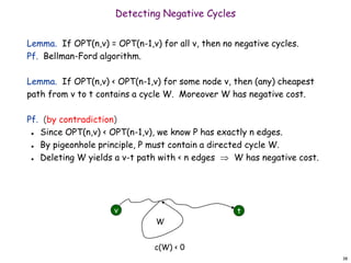
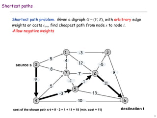
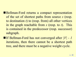
Bellman-Ford is an algorithm for finding shortest paths in a graph with positive or negative edge weights. It uses dynamic programming to iteratively update the shortest path costs from a source node to all other nodes. If the shortest path costs have not converged after |V|-1 iterations, there must be a negative weight cycle present in the graph. The Bellman-Ford algorithm returns both the shortest path costs and a predecessor graph that implicitly represents the shortest paths.

1. 1
Dynamic Programming

2. 6.8 Shortest Paths
WARNING:
Watch for ambiguous use of “shortest”
in the sense of least weight/cost, and
in the sense of fewest edges.

3. 3
Shortest paths
Shortest path problem. Given a digraph G = (V, E), with arbitrary edge
weights or costs cvw, find cheapest path from node s to node t.
•Allow negative weights
7
1 3
source s
-1
8
5
7
5 4
-3
-5
12
10
13
9
cost of the shown path s-t = 9 - 3 + 1 + 11 = 18 (min. cost = 11) destination t
0
4
5
2
6
9
-3
1 11

4. Dijkstra. Can fail if negative edge costs/weights are present.
Re-weighting. Adding a constant to every edge weight can fail.
4
Shortest Paths: Failed Attempts
s t
2 2
-3
3
3
u
t
s v
2
1
3
-6
5 5
6
6
0

5. 5
Negative cycles
Def. A negative cycle is a directed cycle such that the sum of its edge weights is
negative.
-3
5
-3
-4
4
a negative cycle W :

6. 6
Shortest paths and negative cycles
Lemma 1. If some path from v to t contains a negative cycle, then there does not
exist a cheapest path from v to t.
Pf. If there exists such a cycle W, then we can build a v↝t path of arbitrarily
negative weight by detouring around the cycle as many times as desired. ▪
W
c(W) < 0
v t

7. 7
Shortest paths and negative cycles
Lemma 2. If G has no negative cycle, then there exists a cheapest path from v to t
that is simple (and that has ≤ n – 1 edges).
Pf.
・ Consider a cheapest v↝t path P that uses the fewest number of edges.
・ If P contains a cycle W, we can remove portion of P corresponding to W,
obtaining a path with fewer edges, without increasing the cost. ▪
W
c(W) ≥ 0
v t

8. 8
Shortest path and negative cycle problems
Shortest path problem. Given a digraph G = (V, E) with edge weights cvw and no
negative cycles, find cheapest v↝t path for each node v.
Negative cycle problem. Given a digraph G = (V, E) with edge weights cvw, find a
negative cycle (if one exists).
-3
5
-3
-4
4
negative cycle
4
t
1
-3
shortest-paths tree
5
2

9. 9
Shortest paths: dynamic programming
Def. OPT(i, v) = cost of cheapest v↝t path that uses ≤ i edges. (v  t)
 Case 1: Cheapest v↝t path uses ≤ i – 1 edges.
– OPT(i, v) = OPT(i – 1, v)
 Case 2: Cheapest v↝t path uses exactly i edges.
– if (v, w) is first edge, then OPT uses (v, w), and then selects best w↝t
path using i – 1 edges (equivalent to using ≤ i – 1 edges given Case 1).
Observation. If no negative cycles,
OPT(n – 1, v) = cost of cheapest v↝t path.
Pf. By Lemma 2, cheapest v↝t path is simple. ▪
OPT(i, v) =
0 if i = 0
min OPT(i -1, v) ,
(v, w) Î E
min OPT(i -1, w)+cvw
{ }
ì
í
î
ü
ý
þ
otherwise
ì
í
ï
î
ï
∞
optimal substructure property
(proof via exchange argument)

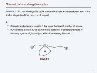
10. 10
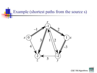
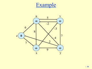
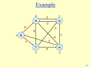
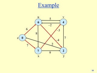
Shortest Paths: Implementation
Analysis. (mn) time, (n2) space.
Shortest-Path(G =(V,E,c), t) {
foreach node v  V
M[0, v]  
M[0, t]  0
for i = 1 to n-1
foreach node v  V
M[i, v]  M[i-1, v]
foreach edge (v, w)  E
M[i, v]  min {M[i, v], cvw + M[i-1, w]}
}

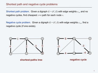
11. Proof of Correctness : A Sketch
Induction Hypothesis: A cheapest path of length k from any
node to node t can be discovered in at most k steps.
Basis Case: k = 0. (t -> t) , k = 1 (single edges v->t).
Induction Step: To construct the cheapest path of length k
from some s (s->v1->*->t), use an edge (s->v1) and the
cheapest path of length k-1 (v1->*->t), discovered using at
most k-1 steps [Ind. Hyp.]. Note that the second foreach-
loop of the nested-loops is run for each edge.
11
…
t
s v1 v2
vk-1

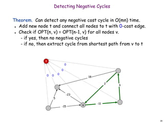
12. 12
Shortest paths: implementation
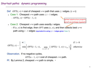
Theorem 1. Given a digraph G = (V, E) with no negative cycles, the
dynamic programming algorithm computes the cost of the cheapest
v↝t path for each node v in Θ(mn) time and Θ(n2) space.
Pf.
 Table requires Θ(n2) space.
 Each iteration i takes Θ(m) time since we examine each edge
once, and the number of iterations is n. ▪
Finding the shortest paths.
 Approach 1: Maintain a successor(i, v) that points to next node on
cheapest v↝t path using at most i edges.
 Approach 2: Compute optimal costs M[i, v] and consider only
edges with M[i, v] = M[i – 1, w] + cvw.

13. 13
Shortest paths: practical improvements
Space optimization. Maintain two 1D arrays (instead of
2D array).
 M(v) = cost of cheapest v↝t path that we have found
so far.
 successor(v) = next node on a v↝t path.
Performance optimization. If M(w) was not updated in
iteration i – 1, then no reason to consider edges entering
w in iteration i.

14. 14
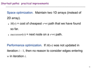
Bellman-Ford: Efficient Implementation
Bellman-Ford(G=(V,E,c), s, t) {
foreach node v  V {
M[v]  
successor[v]  
}
M[t] = 0
for i = 1 to n-1 {
foreach node w  V {
if (M[w] was updated in previous iteration) {
foreach edge (v, w)  E {
if (M[v] > M[w] + cvw) {
M[v]  M[w] + cvw
successor[v]  w
}
}
}
}
If no M[w] value changed in iteration i, stop.
}
}

15. CSE 780 Algorithms
Example (shortest paths from the source s)

16. - 16
Example
0




z
u v
x y
6
5
–3
9
7
7
8
–2
–4
2

17. 17
Example
0

7

6
z
u v
x y
6
5
–3
9
7
7
8
–2
–4
2

18. 18
Example
0
2
7
4
6
z
u v
x y
6
5
–3
9
7
7
8
–2
–4
2

19. 19
Example
0
2
7
4
2
z
u v
x y
6
5
–3
9
7
7
8
–2
–4
2

20. - 20
Example
0
-2
7
4
2
z
u v
x y
6
5
–3
9
7
7
8
–2
–4
2

21. CSE 780 Algorithms
Copyright © The McGraw-Hill Companies, Inc. Permission required for reproduction or display.

22. Bellman-Ford returns a compact representation
of the set of shortest paths from source s (resp.
to destination t) to (resp. from) all other vertices
in the graph reachable from s (resp. to t). This
is contained in the predecessor (resp. successor)
subgraph.
If Bellman-Ford has not converged after |V| - 1
iterations, then there cannot be a shortest path
tree, and there must be a negative weight cycle.
s - 22

23. - 23
Another Look
Note: Bellman-Ford is essentially dynamic programming.
Let d(i, j) = cost of the shortest path from s to i that is at most j hops.
d(i, j) =
0 if i = s  j = 0
 if i  s  j = 0
min({d(k, j–1) + w(k, i): (i,k)  E}
 {d(i, j–1)}) if j > 0
z u v x y
1 2 3 4 5
0 0    
1 0 6  7 
2 0 6 4 7 2
3 0 2 4 7 2
4 0 2 4 7 –2
j
i

24. Claim. ONLY after the ith pass of Bellman-Ford IS d(v) equal to the cost of the cheapest
v↝t path using i edges.
Counterexample. Claim is false!
1
24
Bellman-Ford: analysis
v t
2
d(t) = 0
d(w) = 2
if node w is considered before node v in the 1st pass,
then d(v) = 3 after the 1st pass itself
d(v) = 3
4
w

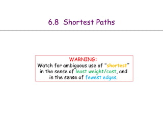
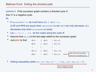
25. 25
Bellman-Ford: analysis
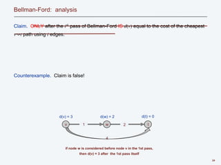
Lemma 3. Throughout Bellman-Ford algorithm, d(v) is the cost of some v↝t path;
after the ith pass, d(v) is no larger than the cost of the cheapest v↝t path using ≤ i
edges.
Pf. [by induction on i]
・ Assume true after ith pass.
・ Let P be any v↝t path (trivially includes the cheapest) with i + 1 edges.
・ Let (v, w) be first edge on path and let P' be subpath from w to t.
・ By inductive hypothesis, d(w) ≤ c(P') since P' is a w↝t path with i edges.
・ After considering v in pass i+1:
Theorem 2. Given a digraph with no negative cycles, Bellman-Ford computes the
costs of the cheapest v↝t paths in O(mn) time and Θ(n) extra space.
Pf. Lemmas 2 + 3. ▪
can be substantially
faster in practice
d(v) ≤ cvw + d(w)
≤ cvw + c(P')
= c(P) ▪

26. 26
Illustrating plausibility of the claim

27. 27
Nodes 2 and 3 are
updated before and
after node 1
Order: t, 1, 2, 3, 1, …

28. 28

29. 29

30. 30
Bellman-Ford: finding the shortest path
Lemma 4. If the successor graph contains a directed cycle W,
then W is a negative cycle.
Pf.
・ If successor(v) = w, we must have d(v) ≥ d(w) + cvw.
(LHS and RHS are equal when successor(v) is set; d(w) can only decrease; d(v)
decreases only when successor(v) is reset)
‣ Let v1 → v2 → … → vk be the nodes along the cycle W.
・ Assume that (vk, v1) is the last edge added to the successor graph.
・ Just prior to that:
‣ Adding inequalities yields c(v1, v2) + c(v2, v3) + … + c(vk–1, vk) + c(vk, v1) < 0. ▪
d(v1) ≥ d(v2) + c(v1, v2)
d(v2) ≥ d(v3) + c(v2, v3)
⋮ ⋮ ⋮
d(vk–1) ≥ d(vk) + c(vk–1, vk)
d(vk) > d(v1) + c(vk, v1)
W is a negative cycle
holds with strict inequality
since we are updating d(vk)

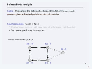
31. 31
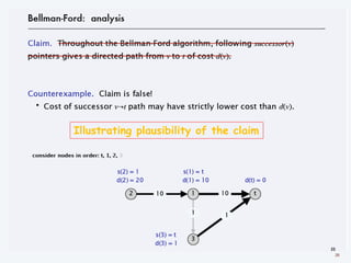
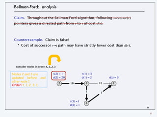
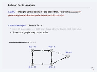
Bellman-Ford: finding the shortest path
Theorem 3. Given a digraph with no negative cycles, Bellman-Ford finds the
cheapest s↝t paths in O(mn) time and Θ(n) extra space.
Pf.
・ The successor graph cannot have a negative cycle. [Lemma 4]
・ Thus, following the successor pointers from s yields a directed path to t.
・ Let s = v1 → v2 → … → vk = t be the nodes along this path P.
・ Upon termination, if successor(v) = w, we must have d(v) = d(w) + cvw.
(LHS and RHS are equal when successor(v) is set; d(·) did not change)
・ Thus,
・
Adding equations yields d(s) = d(t) + c(v1, v2) + c(v2, v3) + … + c(vk–1, vk). ▪
d(v1) = d(v2) + c(v1, v2)
d(v2) = d(v3) + c(v2, v3)
⋮ ⋮ ⋮
d(vk–1) = d(vk) + c(vk–1, vk)
cost of path P
min cost
of any s↝t path
(Theorem 2)
0
since algorithm
terminated

32. Push Pull Alternatives
Current implementation of Bellman-Ford algorithm is pull-
based, where each node polls its neighbors M[…] for
changes.
The efficiency of the algorithm can be improved by
resorting to push-based alternative, where a node
triggers its neighbors when its M[…] changes.
Despite asynchronous updates, the algorithm converges.
32

33. 6.9 Distance Vector Protocol

34. 34
Distance Vector Protocol
Communication network.
 Nodes  routers.
 Edges  direct communication link.
 Cost of edge  delay on link.
Dijkstra's algorithm. Requires global information about the network.
Bellman-Ford. Uses only local information from the neighboring nodes.
Synchronization. We don't expect routers to run in lockstep. The
order in which each foreach loop executes in not important. Moreover,
algorithm still converges even if the updates are asynchronous.
In practice, properties such as locality, compositionality, modularity,
and asynchronous nature are very important.
naturally nonnegative, but Bellman-Ford used anyway!

35. 35
Distance Vector Protocol
Distance vector protocol.
 Each router maintains a vector of shortest path lengths to every
other node (distances) and the first hop on each path (directions).
 Algorithm: each router performs n separate computations, one for
each potential destination node.
 "Routing by rumor."
Ex. RIP, Xerox XNS RIP, Novell's IPX RIP, Cisco's IGRP, DEC's DNA
Phase IV, AppleTalk's RTMP.
Caveat. Edge costs may change during algorithm (or fail completely).
t
v 1
s 1
1
deleted
"counting to infinity"
2 1

36. 36
Path Vector Protocols
Link state routing.
 Each router also stores the entire path.
 Based on Dijkstra's algorithm.
 Avoids "counting-to-infinity" problem and
related difficulties. (see textbook)
 Requires significantly more storage.
Ex. Border Gateway Protocol (BGP), Open
Shortest Path First (OSPF).
not just the distance and first hop

37. 6.10 Negative Cycles in a Graph

38. 38
Detecting Negative Cycles
Lemma. If OPT(n,v) = OPT(n-1,v) for all v, then no negative cycles.
Pf. Bellman-Ford algorithm.
Lemma. If OPT(n,v) < OPT(n-1,v) for some node v, then (any) cheapest
path from v to t contains a cycle W. Moreover W has negative cost.
Pf. (by contradiction)
 Since OPT(n,v) < OPT(n-1,v), we know P has exactly n edges.
 By pigeonhole principle, P must contain a directed cycle W.
 Deleting W yields a v-t path with < n edges  W has negative cost.
v t
W
c(W) < 0

39. 39
Detecting Negative Cycles
Theorem. Can detect any negative cost cycle in O(mn) time.
 Add new node t and connect all nodes to t with 0-cost edge.
 Check if OPT(n, v) = OPT(n-1, v) for all nodes v.
– if yes, then no negative cycles
– if no, then extract cycle from shortest path from v to t
v
18
2
5
-23
-15
-11
6
t
0
0
0
0
0