Download to read offline


![Initialization
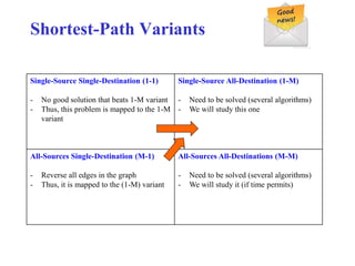
• Maintain d[v] for each v in V
• d[v] is called shortest-path weight estimate
and it is upper bound on δ(s,v)
INIT(G, s)
for each v V do
d[v] ← ∞
π[v] ← NIL
d[s] ← 0
Parent node
Upper bound](https://image.slidesharecdn.com/shortestpath-210915044327/85/Shortest-path-19-320.jpg)
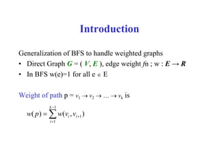
![Relaxation
RELAX(u, v)
if d[v] > d[u]+w(u,v) then
d[v] ← d[u]+w(u,v)
π[v] ← u
5
u v
v
u
2
2
9
5 7
Change d[v]
5
u v
v
u
2
2
6
5 6
When you find an edge (u,v) then
check this condition and relax d[v] if
possible
No chnage](https://image.slidesharecdn.com/shortestpath-210915044327/85/Shortest-path-20-320.jpg)

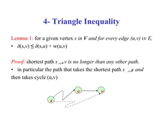
![• Non-negative edge weight
• Like BFS: If all edge weights are equal, then use BFS,
otherwise use this algorithm
• Use Q = min-priority queue keyed on d[v] values
Dijkstra’s Algorithm For Shortest Paths](https://image.slidesharecdn.com/shortestpath-210915044327/85/Shortest-path-22-320.jpg)
![DIJKSTRA(G, s)
INIT(G, s)
S←Ø > set of discovered nodes
Q←V[G]
while Q ≠Ø do
u←EXTRACT-MIN(Q)
S←S U {u}
for each v in Adj[u] do
RELAX(u, v) > May cause
> DECREASE-KEY(Q, v, d[v])
Dijkstra’s Algorithm For Shortest Paths](https://image.slidesharecdn.com/shortestpath-210915044327/85/Shortest-path-23-320.jpg)
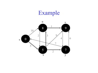
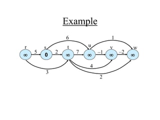
![Example: Initialization Step
3
¥ ¥
¥ ¥
0
s
u v
y
x
10
5
1
2 9
4 6
7
2
DIJKSTRA(G, s)
INIT(G, s)
S←Ø > set of discovered nodes
Q←V[G]
while Q ≠Ø do
u←EXTRACT-MIN(Q)
S←S U {u}
for each v in Adj[u] do
RELAX(u, v) > May cause
> DECREASE-KEY(Q, v, d[v])](https://image.slidesharecdn.com/shortestpath-210915044327/85/Shortest-path-24-320.jpg)

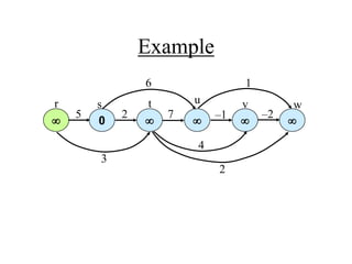
![Example
2
10
5
0
s
u v
y
x
10
5
1
3
9
4 6
7
2
DIJKSTRA(G, s)
INIT(G, s)
S←Ø > set of discovered nodes
Q←V[G]
while Q ≠Ø do
u←EXTRACT-MIN(Q)
S←S U {u}
for each v in Adj[u] do
RELAX(u, v) > May cause
> DECREASE-KEY(Q, v, d[v])](https://image.slidesharecdn.com/shortestpath-210915044327/85/Shortest-path-26-320.jpg)
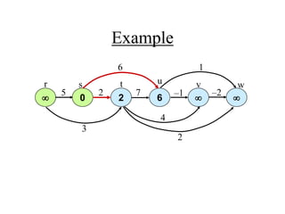
![Example
2
8 14
5 7
0
s
y
x
10
5
1
3 9
4 6
7
2
u v
DIJKSTRA(G, s)
INIT(G, s)
S←Ø > set of discovered nodes
Q←V[G]
while Q ≠Ø do
u←EXTRACT-MIN(Q)
S←S U {u}
for each v in Adj[u] do
RELAX(u, v) > May cause
> DECREASE-KEY(Q, v, d[v])](https://image.slidesharecdn.com/shortestpath-210915044327/85/Shortest-path-27-320.jpg)
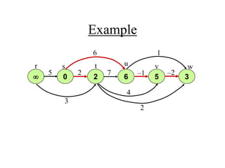
![Example
10
8 13
5 7
0
s
u v
y
x
5
1
2 3 9
4 6
7
2
DIJKSTRA(G, s)
INIT(G, s)
S←Ø > set of discovered nodes
Q←V[G]
while Q ≠Ø do
u←EXTRACT-MIN(Q)
S←S U {u}
for each v in Adj[u] do
RELAX(u, v) > May cause
> DECREASE-KEY(Q, v, d[v])](https://image.slidesharecdn.com/shortestpath-210915044327/85/Shortest-path-28-320.jpg)
![Example
8
u v
9
5 7
0
y
x
10
5
1
2 3 9
4 6
7
2
s
DIJKSTRA(G, s)
INIT(G, s)
S←Ø > set of discovered nodes
Q←V[G]
while Q ≠Ø do
u←EXTRACT-MIN(Q)
S←S U {u}
for each v in Adj[u] do
RELAX(u, v) > May cause
> DECREASE-KEY(Q, v, d[v])](https://image.slidesharecdn.com/shortestpath-210915044327/85/Shortest-path-29-320.jpg)
![Dijkstra’s Algorithm Analysis
DIJKSTRA(G, s)
INIT(G, s)
S←Ø > set of discovered nodes
Q←V[G]
while Q ≠Ø do
u←EXTRACT-MIN(Q)
S←S U {u}
for each v in Adj[u] do
RELAX(u, v) > May cause
> DECREASE-KEY(Q, v, d[v])
O(V)
O(V Log V)
Total in the loop: O(V Log V)
Total in the loop: O(E Log V)
Time Complexity: O (E Log V)](https://image.slidesharecdn.com/shortestpath-210915044327/85/Shortest-path-31-320.jpg)
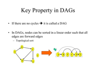
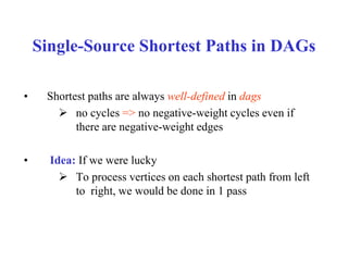
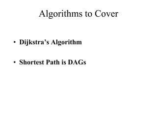
![Single-Source Shortest Paths in DAGs
DAG-SHORTEST PATHS(G, s)
TOPOLOGICALLY-SORT the vertices of G
INIT(G, s)
for each vertex u taken in topologically sorted order do
for each v in Adj[u] do
RELAX(u, v)](https://image.slidesharecdn.com/shortestpath-210915044327/85/Shortest-path-35-320.jpg)


![Single-Source Shortest Paths in
DAGs: Analysis
DAG-SHORTEST PATHS(G, s)
TOPOLOGICALLY-SORT the vertices of G
INIT(G, s)
for each vertex u taken in topologically sorted order do
for each v in Adj[u] do
RELAX(u, v)
O(V+E)
O(V)
Total O(E)
Time Complexity: O (V + E)](https://image.slidesharecdn.com/shortestpath-210915044327/85/Shortest-path-43-320.jpg)

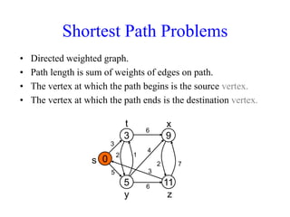
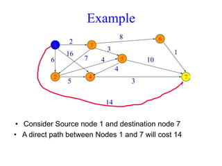
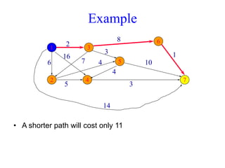
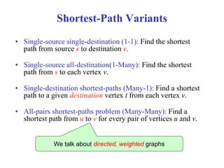
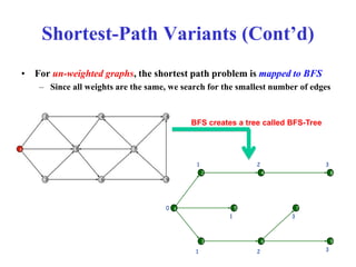
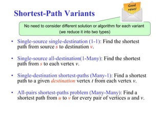
The document discusses shortest path problems in directed weighted graphs, defining various variants such as single-source single-destination, single-source all-destination, and all-pairs shortest-paths. It introduces algorithms like Dijkstra's algorithm for finding shortest paths with non-negative weights and methods for handling graphs with negative-weight edges. Additionally, it emphasizes the optimal substructure property of shortest paths and includes analysis of time complexity for specific algorithms.