Downloaded 394 times

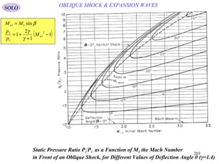
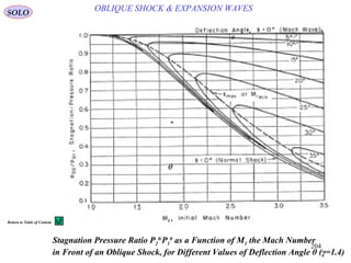
![9
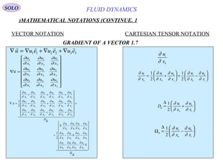
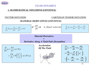
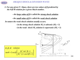
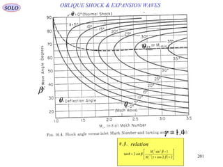
FLUID DYNAMICS
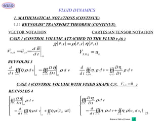
1.MATHEMATICAL NOTATIONS (CONTINUE)
VECTOR NOTATION CARTESIAN TENSOR NOTATION
1.8GAUSS’ THEOREMS (CONTINUE)
( ) ( ) ( )∫∫ ∫∫∫ ⋅∇=⋅
S V
dvAsdAGAUSS
ηη3
( )= ⋅∇ + ∇⋅∫∫∫
A A dvη η
η∇⋅∇ ,A
analytic inV
( )η
∂ η
∂
A ds
A
x
dv
V
k k
k
kS
= ∫∫∫∫∫
∫∫∫
+=
V k
k
k
k
x
A
x
A
∂
∂
η
∂
η∂
↓ = + +
B e e eη η η1 1 2 2 3 3
( ) ( ) ( )[ ]∫∫ ∫∫∫ ⋅∇+∇⋅=⋅
S V
dvABBAsdABGAUSS
4 B A ds A
B
x
B
A
x
dv
V
i k k k
i
k
i
k
kS
= +
∫∫∫∫∫
∂
∂
∂
∂
∇ ×
A analytic inV( ) ∫∫ ∫∫∫ ×∇=×
S V
dvAAsdGAUSS
5 ( )ds A ds A
A
x
A
x
dv
V
i j j i
j
i
i
jS
− = −
∫∫∫∫∫
∂
∂
∂
∂
SOLO](https://image.slidesharecdn.com/fluiddynamics-141022060736-conversion-gate02/85/Fluid-dynamics-9-320.jpg)
![13
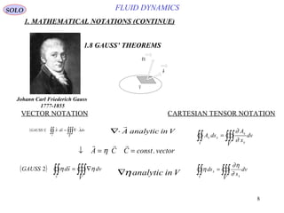
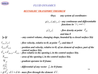
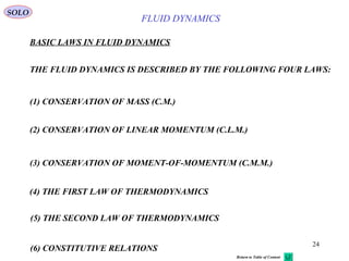
FLUID DYNAMICS
1. MATHEMATICAL NOTATIONS (CONTINUE)
VECTOR NOTATION CARTESIAN TENSOR NOTATION
1.10 MATERIAL DERIVATIVES (CONTINUE)
d u
u
t
dt dr u
= + ⋅∇
∂
∂
du
u
t
dt dx
u
x
i
i
k
i
k
= + ⋅
∂
∂
∂
∂
rdrdDtd
t
u
xd
xd
xd
x
u
x
u
x
u
x
u
x
u
x
u
x
u
x
u
x
u
t
u
t
u
t
u
ud
ud
ud
ikik
Ω++=
+
=
∂
∂
∂
∂
∂
∂
∂
∂
∂
∂
∂
∂
∂
∂
∂
∂
∂
∂
∂
∂
∂
∂
∂
∂
∂
∂
3
2
1
3
3
2
3
1
3
3
2
2
2
1
2
3
1
2
1
1
1
3
2
1
3
2
1
d u
u
t
d t
u
x
u
x
d x
u
x
u
x
d x
i
i
Translation
i
k
k
i
Dilation
k
i
k
k
i
Rotation
k
= +
+ +
+ −
∂
∂
∂
∂
∂
∂
∂
∂
∂
∂
1
2
1
2
( )
( )
( )
( )[ ] Dilationrduu
rdurdu
urdrdurdu
rdurdurdD
T
u
u
ik
⇒⋅∇+∇=
⋅∇+⋅∇=
∇⋅−⋅∇+⋅∇=
××∇−⋅∇=
2
1
2
1
2
1
2
1
2
1
2
1
( )Ωik dr u dr Rotation
= ∇ × × ⇒
1
2
SOLO](https://image.slidesharecdn.com/fluiddynamics-141022060736-conversion-gate02/85/Fluid-dynamics-13-320.jpg)
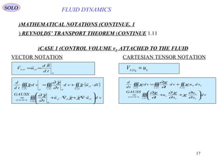
![21
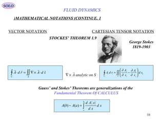
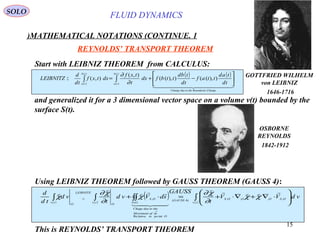
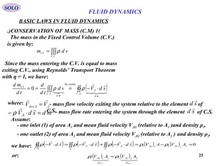
FLUID DYNAMICS
1. MATHEMATICAL NOTATIONS (CONTINUE)
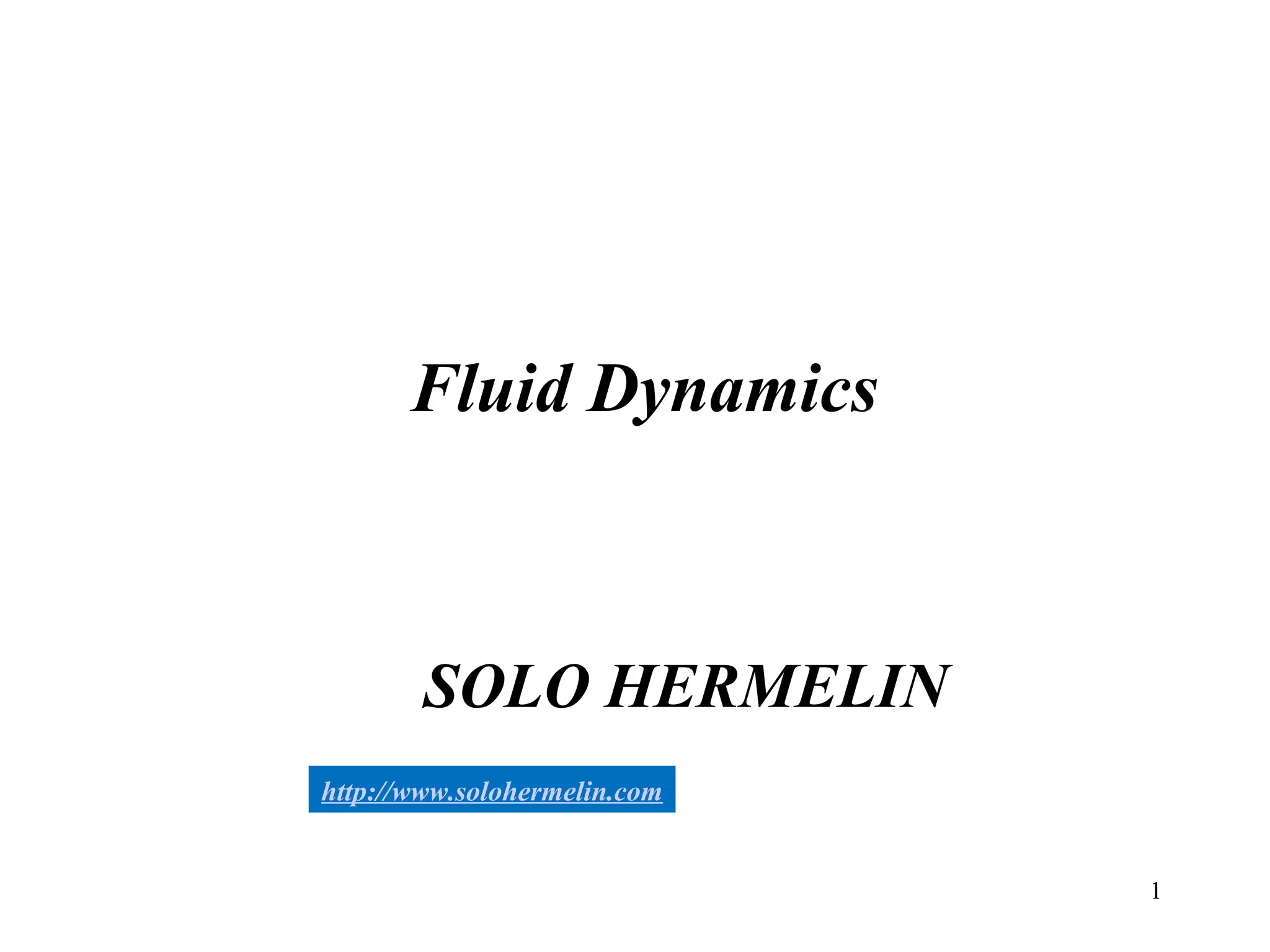
1.11 REYNOLDS’ TRANSPORT THEOREM (CONTINUE)
VECTOR NOTATION CARTESIAN TENSOR NOTATION
We have
( )
( )
( ) ( )[ ]
( )
( )[ ]∫∫∫∫∫=
∫∫
∫∫∫
∫∫
∫∫∫∫∫∫
⋅−+
⋅+
⋅∇+∇⋅−
∇⋅+=
⋅+
⋅∇−=
+
+
)(
,,
)(
4
.
)(
,
)(
,,,,,,
)(
,
)(
,,
)(
tS
OOS
tv
O
MDG
DerMat
GAUSS
tS
OS
tv
OOOOOO
O
tS
OS
tv
OO
OO
tv
sduVvd
tD
D
sdV
vduuu
t
sdV
vdu
t
vd
td
d
ρηρ
η
ρη
ρηηρη
∂
η∂
ρ
ρη
ρηρ
∂
η∂
ρη ( )
( )
( ) ( )
( )
( )[ ]∫∫∫∫∫=
∫∫
∫∫∫
∫∫
∫∫∫∫∫∫
−+
+
+−
+=
+
−=
+
+
)(
,
)(
4
.
)(
,
)(
)(
,
)()(
tS
kkkOSi
tv
i
MDG
DerMat
GAUSS
tS
kkOSi
tv k
k
i
k
i
k
k
i
k
i
tS
kkOSi
tv k
k
i
i
tv
i
sduVvd
tD
D
sdV
vd
x
u
x
u
x
u
t
sdV
vd
x
u
t
vd
td
d
ρηρ
η
ρη
∂
ρ∂
η
∂
η∂
ρ
∂
η∂
∂
η∂
ρ
ρη
∂
ρ∂
ηρ
∂
η∂
ρη
CASE 5 ( ) ( ) ( )
χ ρ ηr t r t r t, , ,≡
SOLO](https://image.slidesharecdn.com/fluiddynamics-141022060736-conversion-gate02/85/Fluid-dynamics-21-320.jpg)
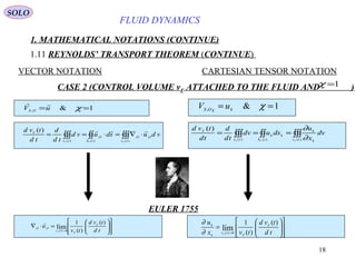
![22
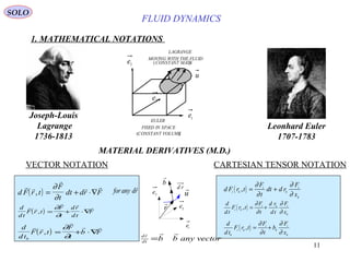
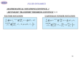
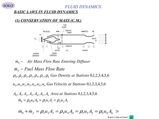
FLUID DYNAMICS
1. MATHEMATICAL NOTATIONS (CONTINUE)
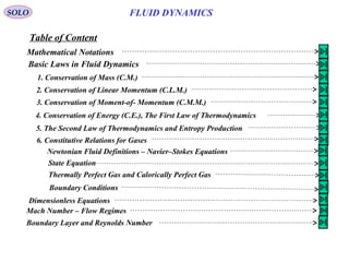
1.11 REYNOLDS’ TRANSPORT THEOREM (CONTINUE)
VECTOR NOTATION CARTESIAN TENSOR NOTATION
REYNOLDS 1
( )[ ]
⋅−+= ∫∫∫∫∫
∫∫∫
)(
,,
)(
)(
tS
OOS
tv
O
O
tv
sduVvd
tD
D
vd
td
d
ρηρ
η
ρη
( )[ ]
−+= ∫∫∫∫∫
∫∫∫
)(
,
)(
)(
tS
kkkOSi
tv
i
tv
i
sduVvd
tD
D
dv
td
d
ρηρ
η
ρη
REYNOLDS 2
( )[ ]
=
⋅−+
∫∫∫
∫∫∫∫∫
)(
)(
,,
)(
tv
O
tS
OSO
O
tv
vd
tD
D
sdVuvd
td
d
ρ
η
ρηρη
( )[ ]
=
−+
∫∫∫
∫∫∫∫∫
)(
)(
,
)(
tv
i
tS
kkOSki
tv
i
vd
tD
D
sdVuvd
td
d
ρ
η
ρηρη
CASE 5 ( ) ( ) ( )
χ ρ ηr t r t r t, , ,≡
SOLO](https://image.slidesharecdn.com/fluiddynamics-141022060736-conversion-gate02/85/Fluid-dynamics-22-320.jpg)
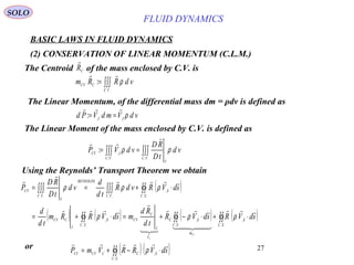
![31
FLUID DYNAMICS
BASIC LAWS IN FLUID DYNAMICS (CONTINUE)
(2.2) CONSERVATION OF LINEAR MOMENTUM (CONTINUE)
VECTOR NOTATION CARTESIAN TENSOR NOTATION
C.L.M.-2
Since this is true for all volumes vF(t) attached to the fluid we can drop the volume integral.
[ ] [ ] [ ]τσ
τρσρ
∂
∂
ρ
∂
∂
ρρ
~~
~~
2
1
,,,
,
2
,
,
.).(
+−=
⋅∇+∇−=⋅∇+=
×∇×−
∇+=
∇⋅+=
Ip
pGG
uuu
t
u
uu
t
u
tD
uD
III
II
I
I
I
DM
I
ikikik
i
ik
i
i
i
ik
i
k
i
k
i
j
jjj
i
i
k
i
k
i
DM
i
p
xx
p
G
x
G
x
u
u
x
u
uuu
xt
u
x
u
u
t
u
tD
uD
τδσ
∂
τ∂
∂
∂
ρ
∂
σ∂
ρ
∂
∂
∂
∂
∂
∂
∂
∂
ρ
∂
∂
∂
∂
ρρ
+−=
+−=+=
⋅−⋅−
+=
⋅+=
2
1
.).(
SOLO
Derivation From Integral Form (Continue)
( )∫∫∫
∫∫∫∫∫∫∫∫
⋅∇+=
⋅+=
)(
,
)()()(
,
~
~
tv
I
tStvtv
I
I
F
FFF
vdG
sdvdGvd
tD
uD
σρ
σρρ
∫∫∫
∫∫∫∫∫∫∫∫
+=
+=
)(
)()()(
tv i
ik
i
tS
kik
tv
i
tv
i
F
FFF
vd
x
G
sdvdGvd
tD
uD
∂
σ∂
ρ
σρρ](https://image.slidesharecdn.com/fluiddynamics-141022060736-conversion-gate02/85/Fluid-dynamics-31-320.jpg)
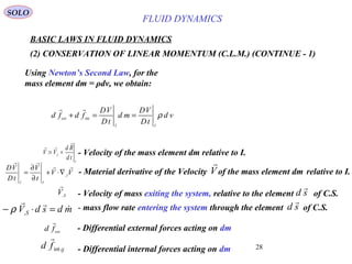
![32
BASIC LAWS IN FLUID DYNAMICS
(2)CONSERVATION OF LINEAR MOMENTUM (C.L.M.)
SOLO
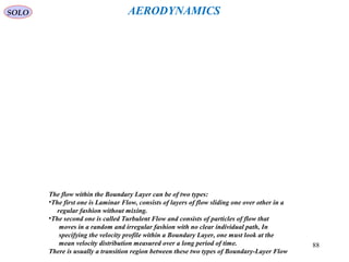
Let compute the C.L.M. in the tangential to the
wheel direction, for the Pelton Water Wheel
( )[ ]
( ) ( )
t
tvtv
extjj RfdfdrVrQVQ −+=−−− ∫∫
0
int
0
cos βωωρρ
where
( ) ( )∫∫∫∫ ⋅−=⋅−=
outin A
S
A
S
sdVsdVQ
,,
: ρρρ
( ) ( )βωρ cos1+−= rVQR jt
Therefore
The average Torque on the water wheel is ( ) ( )βωρ cos1+−== rVrQrRTorque jt
The Power developed is ( ) ( )βωωρω cos1+−==⋅= rVrQrRTorquePower jt
The average Tangential Reaction Force on
the bucket is
In steady-state the directions and
magnitudes of flows are fixed, therefore
0
..
== ∫∫∫
I
VC
I
CV
vdV
td
d
td
Pd
ρ
( ) ( )
∑∑∫∫∫∫∫
∫∫∫∫∫∫∫
=+⋅+=
⋅+=⋅+
−−
ext
j
j
SCVC
SC
md
S
I
CV
SC
md
S
I
VC
FFsdvdg
sdVV
td
Pd
sdVVvdV
td
d
....
..
,
..
,
..
σρ
ρρρ
Example
FLUID DYNAMICS](https://image.slidesharecdn.com/fluiddynamics-141022060736-conversion-gate02/85/Fluid-dynamics-32-320.jpg)
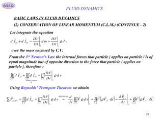
![34
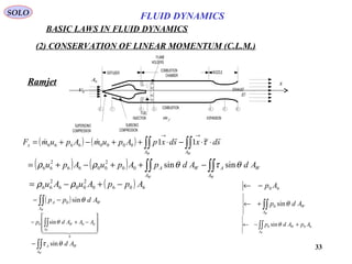
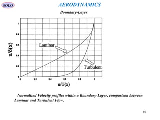
Ramjet
SOLO
CONSERVATION OF LINEAR MOMENTUM (C.L.M.) (continue – 1)
( ) ( )
DRAGFRICTION
A
WA
DRAGPRESURE
A
WA
THRUST
x
WW
AdAdppAppAuAuF ∫∫∫∫ −−−−+−= θτθρρ sinsin06060
2
006
2
66
00000666 & mAummAu f
=+= ρρUsing C.M.
( ) ( ) 0006060
2
006
2
66 umummAppAuAuTHRUST ef
−+=−+−= ρρ
or
we obtain
( )[ ] ( ) 060600 /:1 mmfAppuufmTHRUST fe
=−+−+==T
and ( )
DRAGFRICTION
A
WA
DRAGPRESURE
A
WA
WW
AdAdppDRAGD ∫∫∫∫ +−== θτθ sinsin0
1 2 30 4 5 6
SUPERSONIC
COMPRESSION
SUBSONIC
COMPRESSION
COMBUSTION
FUEL
INJECTION EXPANSION
NOZZLECOMBUSTION
CHAMBER
DIFFUSER
FLAME
HOLDERS
EXHAUST
JET
0V
0A
fm
x
BASIC LAWS IN FLUID DYNAMICS
FLUID DYNAMICS
Return to Table of Content](https://image.slidesharecdn.com/fluiddynamics-141022060736-conversion-gate02/85/Fluid-dynamics-34-320.jpg)
![38
BASIC LAWS IN FLUID DYNAMICS
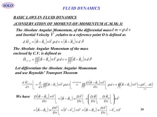
(3) CONSERVATION OF MOMENT-OF-MOMENTUM (C.M.M.)
SOLO
( )
( ) ( ) ( ) ( )
( )
systemoutsidefromexertedTorque
M
l
lz
j
j
tv
ext
AVVrAVVr
SC
S
statesteady
VC
zSnSn
MFrdfrsdVVrvdVr
td
d
∑∑∫∫∫∫ ++=⋅−−
+−−→
θθ
ρρ
θθ
θθ
ρρ
22,21111,122
..
,
0
..
We obtain
( ) ( )[ ] zflow
MQVrVr =− 111122
ρθθ
or
( ) ( ) ( ) ( ) ( ) ( )[ ] ( ) zSnSnSn
MAVVrVrAVVrAVVr =−=− 11,1112211,11122,222
ρρρ θθθθ
Euler Turbine Equation
ρ1 - mean fluid density one inlet (1) of area A1.
where
ρ2 - mean fluid density one outlet (2) of area A2.
(Vθ )1, r1 - mean fluid tangential velocity and radius one inlet (1) of area A1.
(Vθ )2, r2 - mean fluid tangential velocity and radius one outlet (2) of area A2.
(V,Sn )1 - mean fluid normal velocity (relative to A1) one inlet (1) of area A1.
(V,Sn )2 - mean fluid normal velocity (relative to A2) one outlet (2) of area A2.
- mean flow rate one outlet (1) of area A1.( ) 11,1 : AVQ Snflow =
Leonhard Euler
(1707-1783)
FLUID DYNAMICS
Return to Table of Content](https://image.slidesharecdn.com/fluiddynamics-141022060736-conversion-gate02/85/Fluid-dynamics-38-320.jpg)
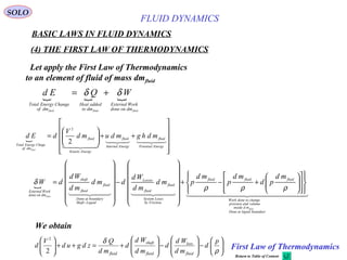
![43
FLUID DYNAMICS
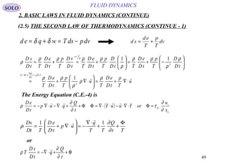
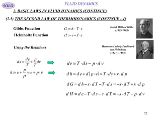
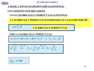
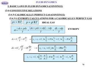
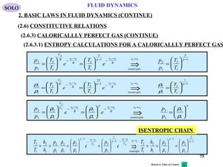
2. BASIC LAWS IN FLUID DYNAMICS (CONTINUE)
(2.4) CONSERVATION OF ENERGY (C.E.)
– THE FIRST LAW OF THERMODYNAMICS (CONTINUE-4)
VECTOR NOTATION CARTESIAN TENSOR NOTATIONC.E.-3
Since the last equation is valid for each vF(t) we can drop the integral and obtain:
( ) ( )
q
t
Q
uGuupue
tD
D
⋅∇−+
⋅+⋅⋅∇+⋅−∇=
+
∂
∂
ρτρ ~
2
1 2 ( ) ( )
k
k
kk
k
iik
k
k
x
q
t
Q
uG
x
u
x
up
ue
tD
D
∂
∂
∂
∂
ρ
∂
τ∂
∂
∂
ρ
−+
++−=
+ 2
2
1
Multiply (C.L.M.-2) by
u
τρρ ~⋅∇⋅+∇⋅−⋅=⋅ upuuG
tD
uD
u
( )
k
ik
i
k
kkk
i
i
x
u
x
p
uuGu
tD
D
tD
uD
u
∂
τ∂
∂
∂
ρρρ +−== 2
Subtract this equation from (C.E.-3)
C.E.-4
( )[ ]ρ τ τ
∂
∂
D e
D t
p u u u
Q
t
q
= − ∇⋅ + ∇⋅ ⋅ − ⋅∇⋅
+ −∇⋅
~ ~
Φ
ρ
∂
∂
τ
∂
∂
∂
∂
∂
∂
D e
D t
p
u
x
u
u
x
Q
t
q
x
k
k
ik
i
k
k
k
=− +
+ −
Φ
( )Φ ≡ ∇⋅ ⋅ − ⋅∇ ⋅ >~ ~τ τ
u u 0
Φ ≡ >τ
∂
∂
ik
i
k
u
x
0
(Proof of inequality given later)
SOLO](https://image.slidesharecdn.com/fluiddynamics-141022060736-conversion-gate02/85/Fluid-dynamics-43-320.jpg)
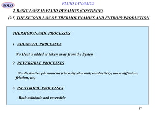
![48
FLUID DYNAMICS
2. BASIC LAWS IN FLUID DYNAMICS (CONTINUE)
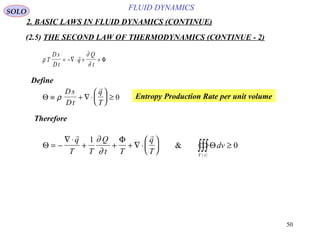
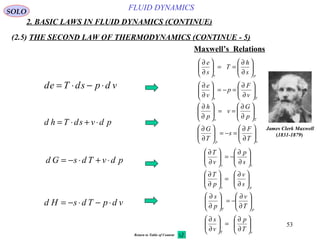
(2.5) THE SECOND LAW OF THERMODYNAMICS AND ENTROPY PRODUCTION
2nd
LAW OF THERMODYNAMICS
Using GAUSS’ THEOREM
0
)()(
≥+ ∫∫∫∫∫
tStv FF
Ad
T
q
vds
td
d
ρ
00
)(
)1(
)()(
≥
⋅∇+⇒≥+ ∫∫∫∫∫∫∫∫
tv
GAUSS
tStv FFF
vd
T
q
tD
sD
Ad
T
q
vd
tD
sD
ρρ
- Change in Entropy per unit volumed s
- Local TemperatureT [ ]K
- Fluid Densityρ [ ]3
/ mKg
d e q w T ds pdv= + = −δ δ d s
d e
T
p
T
dv= +
SOLO
For a Reversible Process
- Rate of Conduction and Radiation of Heat from the System
per unit surface
q
[ ]2
/ mW
Gibbs Relation
Josiah Willard Gibbs
(1839-1903)](https://image.slidesharecdn.com/fluiddynamics-141022060736-conversion-gate02/85/Fluid-dynamics-48-320.jpg)
![54
FLUID DYNAMICS
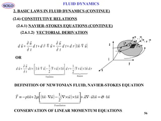
2. BASIC LAWS IN FLUID DYNAMICS (CONTINUE)
(2.6) CONSTITUTIVE RELATIONS FOR GASES
(2.6.1) NEWTONIAN FLUID DEFINITION – NAVIER–STOKES EQUATIONS
[ ] τσ ~~ +−= Ip
Stress
NEWTONIAN FLUID:
The Shear Stress on
A Surface Parallel
to the Flow =
Distance Rate of
Change of Velocity
SOLO
CARTESIAN TENSOR NOTATION
ikikik p τδσ +−=
VECTOR NOTATION
- Stress tensor (force per unit surface) of the surrounding
on the control surface ( )2
/ mN
σ~
- Shear stress tensor (force per unit surface) of the surrounding on the control
surface ( )2
/ mN
τ~](https://image.slidesharecdn.com/fluiddynamics-141022060736-conversion-gate02/85/Fluid-dynamics-54-320.jpg)
![55
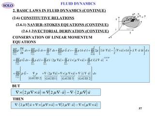
FLUID DYNAMICS
2. BASIC LAWS IN FLUID DYNAMICS (CONTINUE)
(2.6) CONSTITUTIVE RELATIONS
(2.6.1) NEWTONIAN FLUID DEFINITION – NAVIER–STOKES EQUATIONS
M. NAVIER 1822
INCOMPRESSIBLE FLUIDS
(MOLECULAR MODEL)
G.G. STOKES 1845
COMPRESSIBLE FLUIDS
(MACROSCOPIC MODEL)
VECTOR NOTATION CARTESIAN TENSOR NOTATION
[ ] [ ] ( )[ ] [ ]IuuuIpIp
T
∇+∇+∇+−=+−= λµτσ ~~
ik
k
k
i
k
k
i
ikikikik
x
u
x
u
x
u
pp δ
∂
∂
λ
∂
∂
∂
∂
µδτδσ +
++−=+−=
( )[ ] [ ]( ) ( ) ( ) µλλµλµτ
3
2
32~0 −=⇒∇+∇=∇+∇+∇== utrutrIutruutrtr
T
( ) µλ
∂
∂
λµδ
∂
∂
λ
∂
∂
µτ
3
2
0322 −=⇒=+=+=
i
i
ik
k
k
i
i
ii
x
u
x
u
x
u
SOLO
STOKES ASSUMPTION µλ
3
2
−=0~ =τtrace
μ, λ - Lamé parameters from Elasticity](https://image.slidesharecdn.com/fluiddynamics-141022060736-conversion-gate02/85/Fluid-dynamics-55-320.jpg)
![58
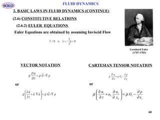
FLUID DYNAMICS
2. BASIC LAWS IN FLUID DYNAMICS (CONTINUE)
I
x
y
z
T n= ⋅~σ
d s n ds=
r
dru
u + du
THEREFORE
( ) ( ) ( ){ }∫∫∫∫∫∫ ⋅∇∇+×∇×∇−⋅∇∇+∇−=
)()(
2
tVtV
vduuupGvd
tD
uD
λµµρρ
OR
( ) ( )[ ]uupG
tD
uD
⋅∇+∇+×∇×∇−∇−= µλµρρ 2
SOLO
(2.6) CONSTITUTIVE RELATIONS
(2.6.1) NAVIER–STOKES EQUATIONS (CONTINUE)
(2.6.1.2)VECTORIAL DERIVATION (CONTINUE)](https://image.slidesharecdn.com/fluiddynamics-141022060736-conversion-gate02/85/Fluid-dynamics-58-320.jpg)
![59
FLUID DYNAMICS
2. BASIC LAWS IN FLUID DYNAMICS (CONTINUE)
VECTOR NOTATION CARTESIAN TENSOR NOTATION
CONSERVATION OF LINEAR MOMENTUM
( ) ( )[ ]∇ ⋅ = − ∇ − ∇ × ∇ × + ∇ + ∇ ⋅~σ µ µ λp u u
2 ( )
++
++−=
k
k
ii
k
k
i
iii
ik
x
u
xx
u
x
u
xx
p
x ∂
∂
λµ
∂
∂
∂
∂
∂
∂
µ
∂
∂
∂
∂
∂
σ∂
2
( ) ( )[ ]
ρ ρ σ
ρ µ µ λ
Du
Dt
G
G p u u
= + ∇ ⋅
= − ∇ − ∇ × ∇ × + ∇ + ∇ ⋅
~
2 ( )
++
++−=
+=
k
k
ii
k
k
i
ii
i
i
ik
i
i
x
u
xx
u
x
u
xx
p
G
x
G
tD
uD
∂
∂
λµ
∂
∂
∂
∂
∂
∂
µ
∂
∂
∂
∂
ρ
∂
σ∂
ρρ
2
USING STOKES ASSUMPTION tr ~τ λ µ= ⇒ = −0
2
3
( )
⋅∇∇+×∇×∇−∇−=
⋅∇+=
uupG
G
tD
uD
µµρ
σρρ
3
4
~
+
++−=
+=
k
k
ki
k
k
i
kk
i
k
ik
i
i
x
u
xx
u
x
u
xx
p
G
x
G
tD
uD
∂
∂
µ
∂
∂
∂
∂
∂
∂
µ
∂
∂
∂
∂
ρ
∂
σ∂
ρρ
3
4
SOLO
(2.6) CONSTITUTIVE RELATIONS
(2.6.1) NAVIER–STOKES EQUATIONS (CONTINUE)](https://image.slidesharecdn.com/fluiddynamics-141022060736-conversion-gate02/85/Fluid-dynamics-59-320.jpg)
![61
FLUID DYNAMICS
2. BASIC LAWS IN FLUID DYNAMICS (CONTINUE)
(2.6.1.3) COMPUTATION
BUT
Φ
Φ = = +
= +
=
=
τ
∂
∂
τ
∂
∂
τ
∂
∂
τ
∂
∂
∂
∂
τ
τ τ
ik
i
k
ik
i
k
ki
k
i
ik
i
k
k
i
ik ik
u
x
u
x
u
x
u
x
u
x
D
ik ki1
2
1
2
τ µ λ δik ik kk ikD D= +2
HENCE ( )Φ = = +τ µ λ δik ik ik kk ik ikD D D D2
OR
( )[ ] ( )[ ]
( )[ ] ( )
Φ = + + + + + + +
+ + + + + + + + + + ⇒
=
2 2
2 2
11 11 22 33 11 22 11 22 33 22
33 11 22 33 33 12
2
21
2
13
2
31
2
23
2
32
2
µ λ µ λ
µ λ µ
D D D D D D D D D D
D D D D D D D D D D D
D Dij ji
( ) ( )Φ = + + + + + + + +2 2 2 211
2
22
2
33
2
12
2
13
2
23
2
11 22 33
2
µ λD D D D D D D D DOR
SOLO
(2.6) CONSTITUTIVE RELATIONS
(2.6.1) NAVIER–STOKES EQUATIONS (CONTINUE)](https://image.slidesharecdn.com/fluiddynamics-141022060736-conversion-gate02/85/Fluid-dynamics-61-320.jpg)
![62
FLUID DYNAMICS
2. BASIC LAWS IN FLUID DYNAMICS (CONTINUE)
(2.6.1.3) COMPUTATION (CONTINUE)
USING STOKES ASSUMPTION: tr ~τ λ µ= ⇒ = −0
2
3
Φ
( ) ( )Φ = + + + + + + + +2 2 2 211
2
22
2
33
2
12
2
13
2
23
2
11 22 33
2
µ λD D D D D D D D D
( ) ( ) ( )
( )
( )
( )
Φ = + + − + + + + +
+ + + − + +
+ +
2
3
4
3
4
3
4
2
3
11 22 33
2
11 22 11 33 22 33 11
2
22
2
33
2
2
12
2
13
2
23
2
11 22 33
2
11
2
22
2
33
2
µ µ µ
µ
µ
λ
µ
D D D D D D D D D D D D
D D D D D D
D D D
OR
( ) ( ) ( )[ ] ( )Φ = − + − + − + + + >
2
3
4 011 22
2
11 33
2
22 33
2
12
2
13
2
23
2µ
µD D D D D D D D D
SOLO
(2.6) CONSTITUTIVE RELATIONS
(2.6.1) NAVIER–STOKES EQUATIONS (CONTINUE)](https://image.slidesharecdn.com/fluiddynamics-141022060736-conversion-gate02/85/Fluid-dynamics-62-320.jpg)
![63
FLUID DYNAMICS
2. BASIC LAWS IN FLUID DYNAMICS (CONTINUE)
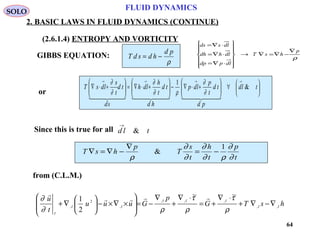
(2.6.1.4) ENTROPY AND VORTICITY
From (C.L.M.)
or
( ) ( )[ ]Du
Dt
u
t
u
u u G p u u
= + ∇
− × ∇ × = − ∇ − ∇ × ∇ × + ∇ + ∇ ⋅
∂
∂ ρ ρ
µ
ρ
λ µ
2
2
1 1 1
2
GIBBS EQUATION: T d s d h
d p
= −
ρ
∀
+⋅∇−
+⋅∇=
+⋅∇
→→→→
tld
pd
td
t
p
ldp
hd
td
t
h
ldh
sd
td
t
s
ldsT &
1
∂
∂
ρ∂
∂
∂
∂
Since this is true for d l t
→
&
T s h
p
T
s
t
h
t
p
t
∇ = ∇ −
∇
= −
ρ
∂
∂
∂
∂ ρ
∂
∂
&
1
SOLO
(2.6) CONSTITUTIVE RELATIONS
(2.6.1) NAVIER–STOKES EQUATIONS (CONTINUE)
Josiah Willard Gibbs
(1903 – 1839)](https://image.slidesharecdn.com/fluiddynamics-141022060736-conversion-gate02/85/Fluid-dynamics-63-320.jpg)
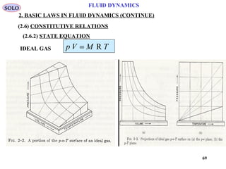
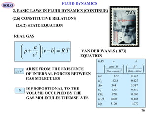
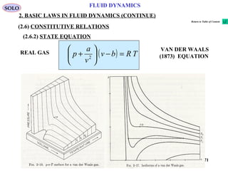
![68
FLUID DYNAMICS
2. BASIC LAWS IN FLUID DYNAMICS (CONTINUE)
(2.6) CONSTITUTIVE RELATIONS
(2.6.2) STATE EQUATION
p - PRESSURE (FORCE / SURFACE)
V - VOLUME OF GAS
M - MASS OF GAS
R - 8314
- 286.9
T - GAS TEMPERATURE
- GAS DENSITY
[ ]m3
[ ]kg
[ ]J kg mol Ko
/ ( )⋅
[ ]J kg Ko
/ ( )⋅R
[ ]kgmol /−η
[ ]o
K
[ ]kg m/ 3
ρ
[ ]2
/ mN
IDEAL GAS
TRMVp η=
TMVp R=
DEFINE: ρ
ρ
= = =
∆ ∆M
V
v
V
M
&
1
pv T= R
p T= ρ R
OR
SOLO](https://image.slidesharecdn.com/fluiddynamics-141022060736-conversion-gate02/85/Fluid-dynamics-68-320.jpg)
![82
SOLO
Dimensionless Equations
Constitutive Relations
TRp ρ=
2
2
1
uTCH p +=
Tkq ∇−=
TCh p=
−
== 2
00
2
00
2
00
1
U
TC
U
TC
C
R
U
p pp
p ρ
ρ
γ
γ
ρ
ρ
ρ
=
2
0
2
0 U
TC
U
h p
2
0
2
0
2
0 2
1
+
=
U
u
U
TC
U
H p
( )
∇
−= 2
0
0
00
0
000
0
3
00 U
TC
l
k
k
C
k
UlU
q p
p µρ
µ
ρ
( ) [ ]3
3
2~ Iuuu T
⋅∇−∇+∇= µµτ [ ]3
0
0
0000
0
0
0
0
0
0000
0
00 3
2~
I
U
u
l
UlU
u
l
U
u
l
UlU
T
⋅∇
−
∇+∇
=
µ
µ
ρ
µ
µ
µ
ρ
µ
ρ
τ
0/~ ρρρ = 0/
~
Uuu = gGG /
~
= ( )2
00/~ Upp ρ=
0/~ lUtt =
2
0/
~
UCTT p=( )2
00/~ Uρττ =
2
0/
~
UHH =
2
0/
~
Uhh =
2
0/~ Uee = ( )2
00/~ Uqq ρ= ( )2
/
~
UQQ =
∇=∇ 0
~
l
0/~ ρρρ = 0/
~
Uuu = gGG /
~
= ( )2
00/~ Upp ρ=
0/~ lUtt =
2
0/
~
UCTT p=( )2
00/~ Uρττ =
2
0/
~
UHH =
2
0/
~
Uhh =
2
0/~ Uee = ( )2
00/~ Uqq ρ= ( )2
/
~
UQQ =
∇=∇ 0
~
l
0/~ µµµ =
0/
~
kkk =
Dimensionless Variables are:
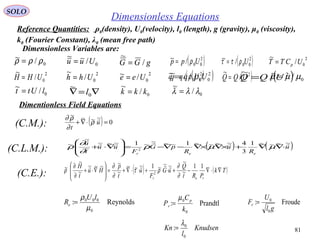
Reference Quantities: ρ0(density), U0(velocity), l0 (length), g (gravity), μ0 (viscosity),
k0 (Fourier Constant), λ0 (mean free path)
0/
~
λλλ =](https://image.slidesharecdn.com/fluiddynamics-141022060736-conversion-gate02/85/Fluid-dynamics-82-320.jpg)
![83
SOLO
Dimensionless Equations
Dimensionless Constitutive Relations
2~
2
1~~
uTH +=
Tp
~~1~ ρ
γ
γ −
= Ideal Gas
( ) [ ]3
~~~
3
2~~~~~~~ Iu
R
uu
R e
T
e
⋅∇−∇+∇=
µµ
τ Navier-Stokes
Th
~~
= Calorically Perfect Gas
Tk
PR
q
re
~~~11~
∇−=
Fourier Law
Reynolds:
0
000
µ
ρ lU
Re =
Prandtl:
0
0
k
C
P
p
r
µ
=
0/~ ρρρ = 0/
~
Uuu = gGG /
~
= ( )2
00/~ Upp ρ=
0/~ lUtt =
2
0/
~
UCTT p=( )2
00/~ Uρττ =
2
0/
~
UHH =
2
0/
~
Uhh =
2
0/~ Uee = ( )2
00/~ Uqq ρ= ( )2
/
~
UQQ =
∇=∇ 0
~
l
0/~ ρρρ = 0/
~
Uuu = gGG /
~
= ( )2
00/~ Upp ρ=
0/~ lUtt =
2
0/
~
UCTT p=( )2
00/~ Uρττ =
2
0/
~
UHH =
2
0/
~
Uhh =
2
0/~ Uee = ( )2
00/~ Uqq ρ= ( )2
/
~
UQQ =
∇=∇ 0
~
l
0/~ µµµ =
0/
~
kkk =
Dimensionless Variables are:
Reference Quantities: ρ0(density), U0(velocity), l0 (length), g (gravity), μ0 (viscosity),
k0 (Fourier Constant), λ0 (mean free path)
0/
~
λλλ =
Return to Table of Content](https://image.slidesharecdn.com/fluiddynamics-141022060736-conversion-gate02/85/Fluid-dynamics-83-320.jpg)
![84
SOLO
Mach Number
Mach number (M or Ma) / is a dimensionless quantity representing
the ratio of speed of an object moving through a fluid and the local
speed of sound.
• M is the Mach number,
• U0 is the velocity of the source relative to the medium, and
• a0 is the speed of sound
Mach:
0
0
a
U
M =
The Mach number is named after Austrian physicist and philosopher
Ernst Mach, a designation proposed by aeronautical engineer Jakob
Ackeret.
Ernst Mach
(1838–1916)
Jakob Ackeret
(1898–1981)
m
Tk
Mo
TR
a Bγγ
==0
• R is the Universal gas constant, (in SI, 8.314 47215 J K−1
mol−1
), [M1
L2
T−2
θ−1
'mol'−1
]
• γ is the rate of specific heat constants Cp/Cv and is dimensionless
γair = 1.4.
• T is the thermodynamic temperature [θ1
]
• Mo is the molar mass, [M1
'mol'−1
]
• m is the molecular mass, [M1
]
AERODYNAMICS](https://image.slidesharecdn.com/fluiddynamics-141022060736-conversion-gate02/85/Fluid-dynamics-84-320.jpg)
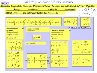
![102
SOLO
Steady One-Dimensional Flow
∂
∂ t
=
0
∂
∂
∂
∂x x2 3
0= =
Flow between two Equilibrium States (1) and (2)
u
p
ρ
T
e
u
p
ρ
T
e
τ 11
q
Q
1
1
1
1
1
2
2
2
2
2
1 2
τ µ
∂
∂
∂
∂
µ
∂
∂
δik
i
k
k
i
k
k
ik
u
x
u
x
u
x
= +
−
2
3
Assume Newtonian fluid (Navier-Stokes Eq.) in each state
( ) ( )
τ µ
∂
∂
τ τ µ
∂
∂
∂
∂
∂
∂
11
1
1
22 33
1
1
1
1 2
1
4
3
2
3
0
=
= =−
=−
⇐ =
⇔
u
x
u
x
q K
T
x
x
equilibrium
We obtain
Let integrate the field equations between state (1) and state (2)
[ ]ρu
1
2
0=
[ ]
ρ τ ρu p G dx2
1
2
12
1
2
1
1
2
0
+ − = ∫
[ ] ( )ρ τ ρuH q u G u Q dx1
2
11
1
2
1
1
2
0 0
+ −
= +∫
No. Equations Unknowns Knowns
ρ2 2,u ρ1 1,u1
1
1
p2
p G1 1,
H2 H1
3 4
STEADY ONE-DIMENSIONAL FLOW EQUATIONS](https://image.slidesharecdn.com/fluiddynamics-141022060736-conversion-gate02/85/Fluid-dynamics-102-320.jpg)

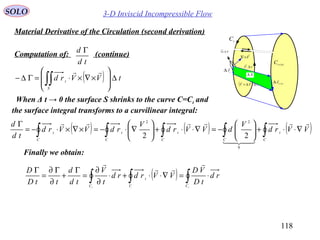
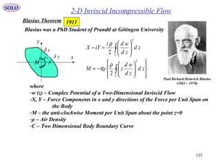
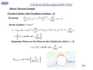
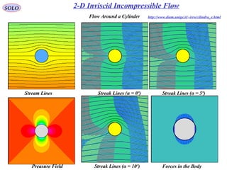
![128
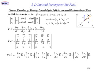
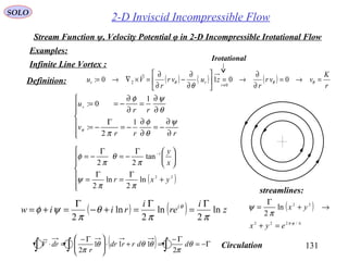
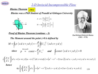
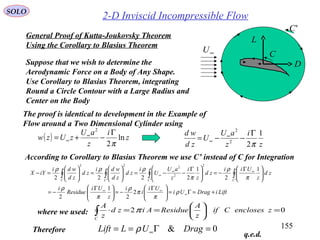
2-D Inviscid Incompressible Flow
In 2-D the velocity vector
SOLO
Stream Function ψ, Velocity Potential φ in 2-D Incompressible Irrotational Flow
x
y V
u
v
ru
θv
r
θ
θθ 1111 vruyvxuV r
+=+=
−
=
v
u
v
ur
θθ
θθ
θ cossin
sincos ( ) θ
θ
i
r
eviuviu +=+
( ) θ
θ
i
r
eviuviu −
+=+
00 222
=∇⋅∇→∇=+=⋅∇ φφuu
2-D Incompressible:
2-D Irrotational:
( )
( ) ( ) ( )ψψψ
ψψ
222
0
222
222
1110
110
∇⋅∇−∇∇⋅=×∇×∇=
→×∇=×∇=+=×∇
zzz
zzuu
0
2
2
2
2
=∇=∇ ψφ
Complex Potential in 2-D Incompressible-Irrotational Flow:
( ) ( ) ( )
yixz
yxiyxzw
+=
+= ,,: ψφ
( ) =
zd
zwd
x
i
x ∂
∂
+
∂
∂ ψφ
yy
i
∂
∂
+
∂
∂
−
ψφ0=x
0=y
( )[ ] ( ) θ
θ
θ
θ
i
r
i
r
eviueviuVviu −∗∗
−=+==−
zd
wd
viu =− θ
θ
i
r e
zd
wd
viu =−
xyyx ∂
∂
−=
∂
∂
∂
∂
=
∂
∂ ψφψφ
Cauchy-Riemann Equations
We found:](https://image.slidesharecdn.com/fluiddynamics-141022060736-conversion-gate02/85/Fluid-dynamics-128-320.jpg)
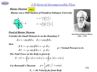
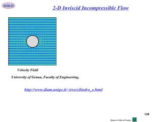
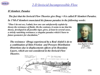
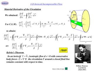
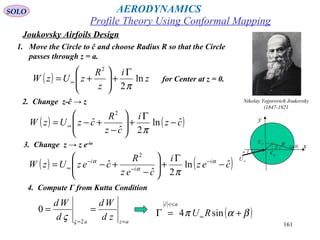
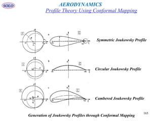
![159
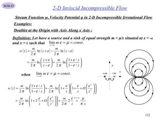
Kutta-Joukovsky
Nikolay Yegorovich Joukovsky
(1847-1921
( ) ( ) ( )cez
i
cez
R
cezUzw i
i
i
ˆln
2ˆ
ˆ
2
−
Γ
+
−
+−= −
−
−
∞
α
α
α
π
( )
viu
cez
i
cez
R
Ue
zd
wd
ii
i
−=
−
Γ
+
−
−= −−∞
−
ˆ
1
2ˆ
1 2
2
αα
α
π
we have
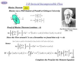
Kutta Condition: The Flow Leaves Smoothly from the Trailing Edge.
This is an Empirical Observation that results from the tendency of
Viscous Boundary Layer to Separate at Trailing Edge.
Martin Wilhelm Kutta
(1867 – 1944)
( )
( )
( ) yx
i
ii
i
az
az
caBcaA
BiA
i
BiA
R
Ue
cea
i
cea
R
Ue
zd
wd
ivu
+=−=
−
Γ
+
−
−=
−
Γ
+
−
−===−
∞
−
−−∞
−
=
=
αα
π
π
α
αα
α
sin:,cos:
1
2
1
ˆ
1
2ˆ
10
2
2
2
2
( ) ( )[ ] ( ) ( )
( )
+
Γ
++−+
Γ
+−−−+
=
∞∞
−
222
22222222222
2
2
2
BA
BAAURBAiBABBARBAU
e i ππα
Profile Theory Using Conformal Mapping
AERODYNAMICSSOLO
Return to Table of Content](https://image.slidesharecdn.com/fluiddynamics-141022060736-conversion-gate02/85/Fluid-dynamics-159-320.jpg)
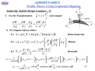
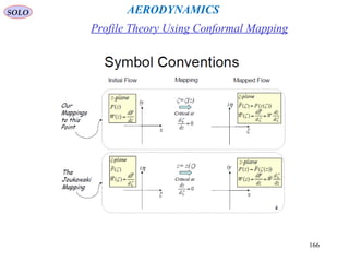
![160
we have
( ) ( )[ ] ( ) ( )
( )
+
Γ
++−+
Γ
+−−−+
==
∞∞
−
=
222
22222222222
2
2
2
0
BA
BAAURBAiBABBARBAU
e
zd
wd i
az
ππα
( ) βααβαα sinsinsin:,coscoscos: RacaBRaacaA yx +=+=−−=−=
( ) ( )
( ) ( )[ ] 222
2222
coscos2cos12
sinsincoscos
RRaRa
RaaRaBA
≈−−++−=
++−+=+
ββαα
βαβα
( ) π2
20 222 Γ
++−= ∞ BAAURBA ( )βαπππ sinsin444 22
2
RaUUBUB
BA
R
+=≈
+
=Γ ∞∞∞
( ) ( )[ ] ( ) ( ) ( )[ ]
( ) ( )[ ] ( )( ) 0
2
2
22222222222
2222222222222222
≈−++=+−+=
−−−+=
Γ
+−−−+
∞∞
∞∞∞
RBABAUBARBAU
URBBARBAUBABBARBAU
π
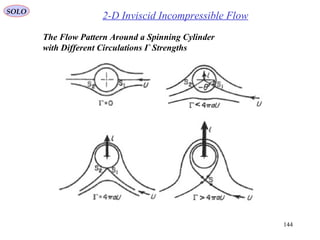
Let check
For this value of Γ, we have
This value of Γ satisfies the Kutta Condition
0=
=az
zd
wd
Joukovsky Airfoils
Profile Theory Using Conformal Mapping
AERODYNAMICSSOLO](https://image.slidesharecdn.com/fluiddynamics-141022060736-conversion-gate02/85/Fluid-dynamics-160-320.jpg)

![192
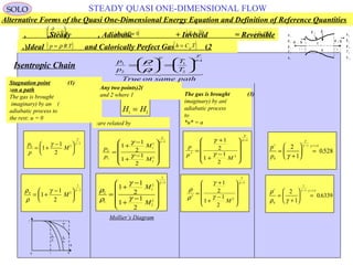
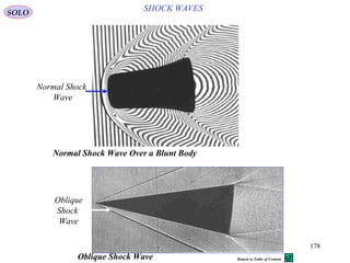
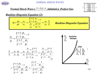
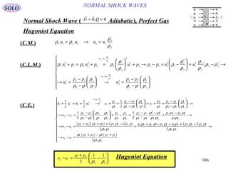
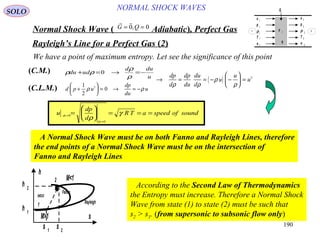
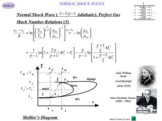
NORMAL SHOCK WAVESSOLO
Normal Shock Wave ) Adiabatic(, Perfect Gas
G Q= =0 0,
Mach Number Relations )2(
( ) ( ) ( ) ( )
( )
( )
( )
( )
( )[ ]
( )( ) ( )
M
M
M
M
M
M
M
M
M
2
2
2
2
1
1
2
1
2
1
2
1
2
1
2
2
1
1
2
1 1
2
1
1
1 2
1
2 1 2
1 1 1 1 1
1
2
=
+
− −
=
+ − −
=
+
+
− +
− −
=
− +
+ / + − / / + − / + − −
∗
=
∗
∗
∗
γ
γ γ γ
γ
γ
γ
γ
γ
γ γ γ γ γ
or
( )
M
M
M
M
M
H H
A A
2
1
2
1
2
1
2
1
21 2
1 2
1
1
2
1
2
2
1
1
1
2
1
2
1
1
=
+
−
−
−
=
+
+
−
+
+
−
=
=
γ
γ
γ γ
γ
γ
γ
( )
( )
ρ
ρ
γ
γ
2
1
1
2
1
2
1 2
1
2
2 1
2 1
2
1
2
1 2 1
1 2
= = = = =
+
− +
=
∗
∗
A A u
u
u
u u
u
a
M
M
M
u
p
ρ
T
e
u
p
ρ
T
e
τ 11
q
Q
1
1
1
1
1
2
2
2
2
2
1 2](https://image.slidesharecdn.com/fluiddynamics-141022060736-conversion-gate02/85/Fluid-dynamics-192-320.jpg)
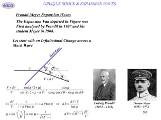
![197
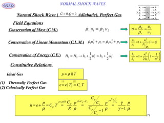
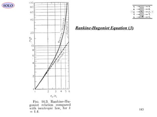
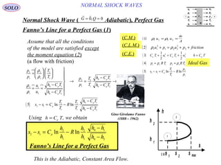
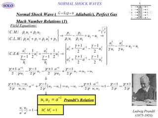
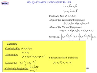
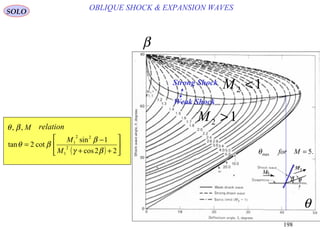
OBLIQUE SHOCK & EXPANSION WAVESSOLO
For a calorically Perfect Gas
( )
( )
( )
( )[ ]
( )[ ]
2
1
1
2
1
2
2
1
2
12
2
2
1
1
2
2
1
2
1
1
2
11/2
1/2
1
1
2
1
21
1
ρ
ρ
γγ
γ
γ
γ
γ
γ
ρ
ρ
p
p
T
T
M
M
M
M
p
p
M
M
n
n
n
n
n
n
=
−−
−+
=
−
+
+=
+−
+
=
βsin11 MMn =
( )θβ −
=
sin
2
2
nM
M
Now we can compute
( )
( ) ( )
( )
( )
( )
⋅+
−
=
−
+
−+
===
−
⇒
=
=−
=
θββ
θβ
β
θβ
βγ
βγ
ρ
ρ
β
θβ
θβ
β
tantan1tan
tantan
tan
tan
sin1
sin12
tan
tan
tan
tan
22
1
22
1
2
1
1
2
12
2
2
1
1
M
M
u
u
ww
w
u
w
u](https://image.slidesharecdn.com/fluiddynamics-141022060736-conversion-gate02/85/Fluid-dynamics-197-320.jpg)
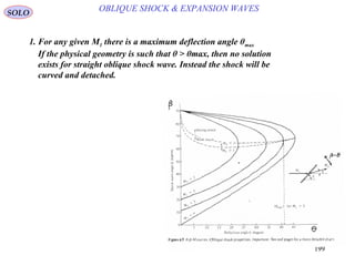
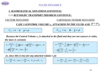
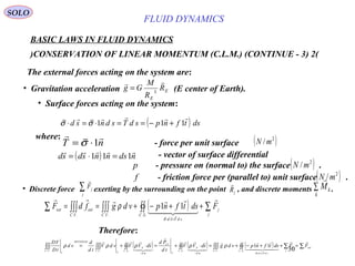
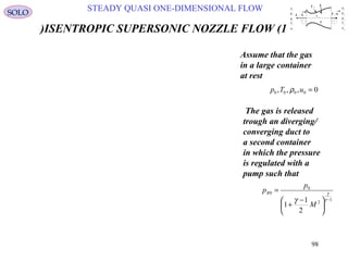
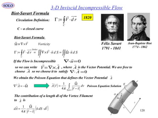
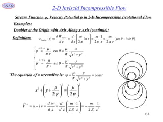
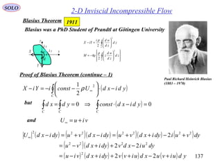
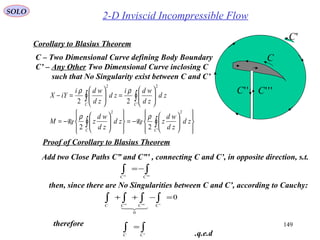
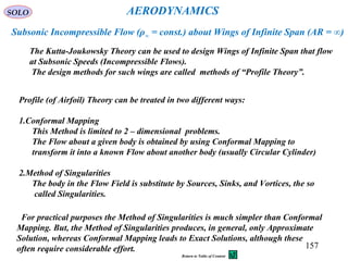
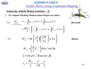
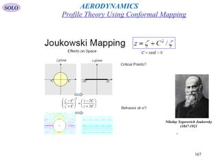
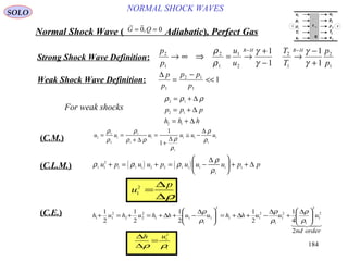
![202
( )[ ]
( )[ ]
( )θβ
γγ
γ
β
−
=
−−
−+
=
=
sin
11/2
1/2
sin
2
2
2
1
2
12
2
11
n
n
n
n
n
M
M
M
M
M
MM
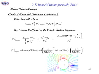
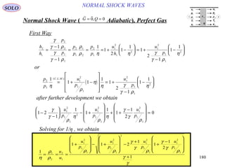
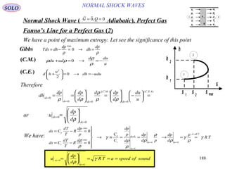
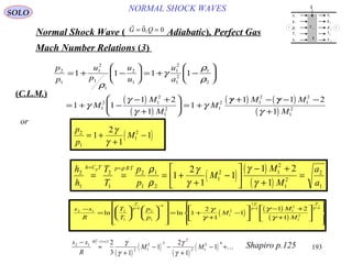
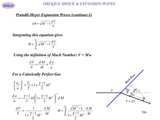
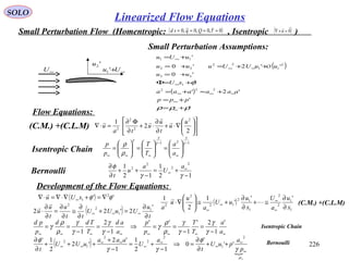
SOLO
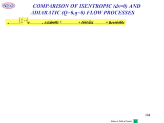
θ
maxθ
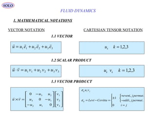
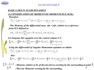
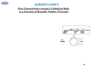
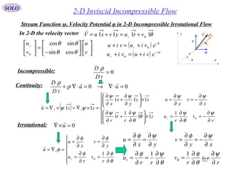
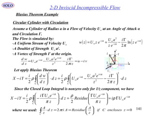
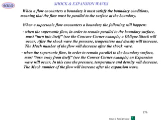
OBLIQUE SHOCK & EXPANSION WAVES
Mach Number in Back of Oblique Shock M2 as a Function of the Mach Number
in Front of the Shock M , for Different Values of Deflection Angle θ (γ=1.4)](https://image.slidesharecdn.com/fluiddynamics-141022060736-conversion-gate02/85/Fluid-dynamics-202-320.jpg)
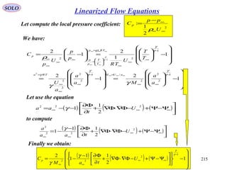
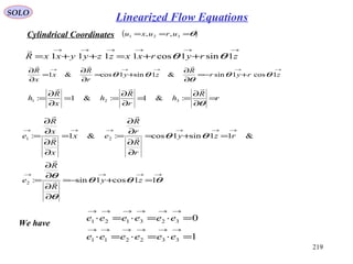
![211
SOLO
For an isentropic ideal gas we have
2
2
11 a
ad
T
Tdd
p
pd
−
=
−
==
γ
γ
γ
γ
ρ
ρ
γ
where
ρ
γ
γ
ρρ
p
TR
d
pdp
a
s
===
∂
∂
=2
is the square of the speed of sound
In this case
2
2
2
1
1
1 2
ad
a
adppd
RTa
RTp
−
=
−
=
=
=
γργ
γ
ρ γ
ρ
and
[ ]222
1
1
1
1
2
2
∞−
−
=
−
= ∫∫
∞∞
aaad
pd
a
a
p
p
γγρ
Using the Bernoulli’s Equation we obtain
( ) ( ) ( ) ( )
Ψ−Ψ+−+
∂
Φ∂
−−=−=− ∞∞∞ ∫
∞
2222
2
1
11 Uu
t
dp
aa
p
p
γ
ρ
γ
( )
2
1
2
2
1
2
2
1
2
1
0
Ψ+++
∂
Φ∂
=
Ψ∇++
+Φ
∂
∂
= ∫∫
∞
p
p
pd
u
t
pd
udd
t ρρ
Bernoulli’s Equation
for Irrotational
and Inviscid Flow
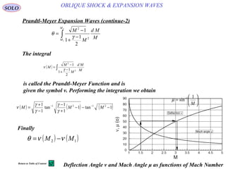
Linearized Flow Equations](https://image.slidesharecdn.com/fluiddynamics-141022060736-conversion-gate02/85/Fluid-dynamics-211-320.jpg)
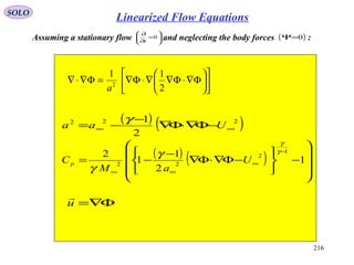
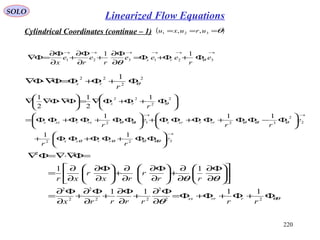
![212
SOLO
Let use the conservation of mass (C.M.) equation
(C.M.) 0=⋅∇+ u
tD
D
ρ
ρ
or
tD
D
u
ρ
ρ
1
−=⋅∇
Let go back to Bernoulli’s Equation ( ) ( )
Ψ−Ψ+−+
∂
Φ∂
−= ∞∞∫
∞
22
2
1
Uu
t
pd
p
p
ρ
and use the Leibnitz rule of differentiation: ( ) ( )uxFdxuxF
xd
d
x
x
,,
0
=∫
to obtain
ρρ
1
=∫
∞
p
p
pd
pd
d
Now we can compute tD
Da
tD
D
d
pd
tD
pD
tD
pDpd
pd
dpd
tD
D
p
p
p
p
ρ
ρ
ρ
ρρρρρ
2
11
===
= ∫∫
∞∞
Therefore ( ) ( )
Ψ−Ψ+−+
∂
Φ∂
=−=−=⋅∇ ∞∞∫
∞
22
22
2
1111
Uu
ttD
D
a
pd
tD
D
atD
D
u
p
p
ρ
ρ
ρ
Since ( )[ ] 0=Ψ−Ψ= ∞∞
tD
D
u
tD
D
we have
∇⋅+
∂
∂
⋅+
∂
Φ∂
=
∇⋅+
∂
Φ∂
∇⋅+
∂
∂
⋅+
∂
Φ∂
=
=
+
∂
Φ∂
∇⋅+
∂
∂
=
+
∂
Φ∂
=⋅∇
Φ∇=
2
2
1
2
1
2
11
2
11
2
2
2
2
2
2
2
2
2
2
2
2
u
u
t
u
u
ta
u
u
t
u
t
u
u
ta
u
t
u
ta
u
ttD
D
a
u
u
GOTTFRIED WILHELM
von LEIBNIZ
1646-1716
Linearized Flow Equations](https://image.slidesharecdn.com/fluiddynamics-141022060736-conversion-gate02/85/Fluid-dynamics-212-320.jpg)
![224
Linearized Flow EquationsSOLO
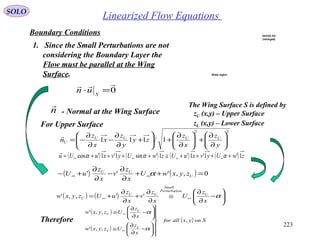
Boundary Conditions (continue -1)
1. Flow must be parallel at the Wing Surface.
The Wing Surface S is defined by
zU (x,y) – Upper Surface
zL (x,y) – Lower Surface
Since the Small Perturbation gives
Linear Equation we can divide the
Airfoil in the Camber Distribution zC (x,y)
and the Thickness Distribution zt (x,y) by:
( )
( )
( ) Sonyxallfor
x
z
Uyxw
x
z
Uyxw
C
C
t
t
,
0,,'
0,,'
−
∂
∂
=
∂
∂
±=±
∞
∞
α
( ) ( ) ( )
( ) ( ) ( )
( ) ( ) ( )[ ]
( ) ( ) ( )[ ]
−=
+=
⇔
−=
+=
2/,,,
2/,,,
,,,
,,,
yxzyxzyxz
yxzyxzyxz
yxzyxzyxz
yxzyxzyxz
LUt
LUC
tCL
tCU
Because of the Linearity the complete solution can be obtained by summing the
Solutions for the following Boundary Conditions
Superposition of
• Angle of Attack
•Camber Distribution
•Thickness Distribution
Section AA
(enlarged)
Wake region
( ) ( ) ( )
( ) ( ) ( )
( ) Sonyxallfor
x
z
x
z
Uyxwyxwyxw
x
z
x
z
Uyxwyxwyxw
tC
tCL
tC
tCU
,
0,,'0,,'0,,'
0,,'0,,'0,,'
∂
∂
−−
∂
∂
=−+=±
∂
∂
+−
∂
∂
=++=±
∞
∞
α
α](https://image.slidesharecdn.com/fluiddynamics-141022060736-conversion-gate02/85/Fluid-dynamics-224-320.jpg)
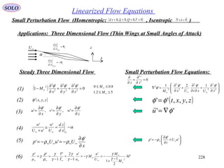
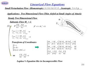
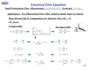
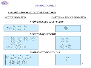
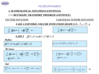
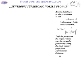
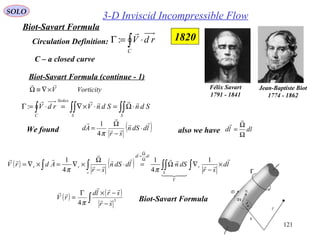
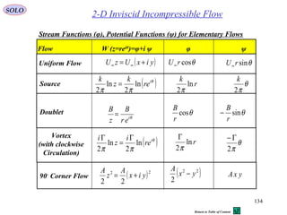
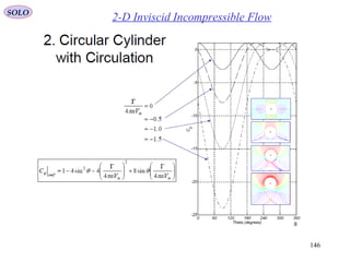
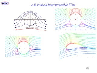
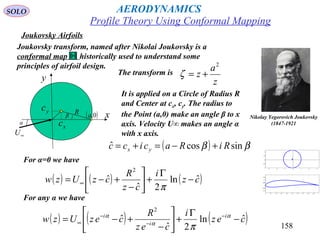
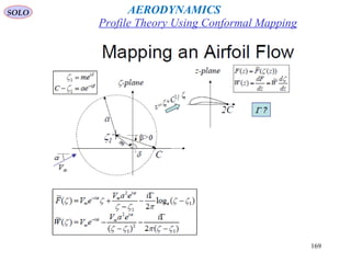
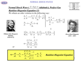
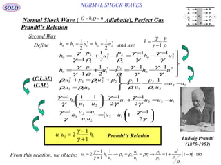
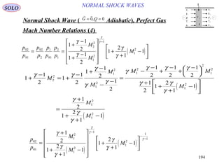
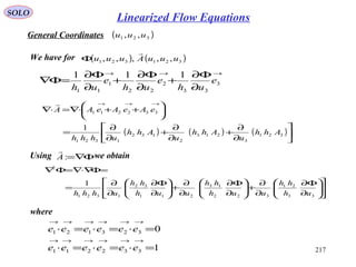
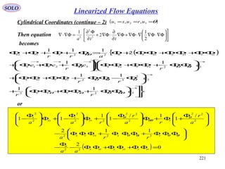
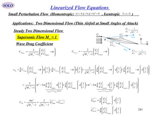
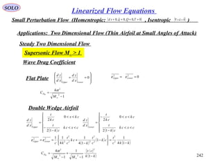
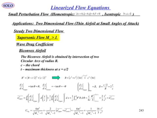
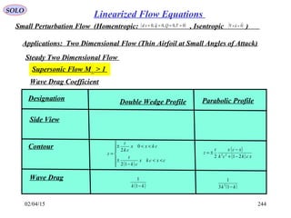
![SOLO
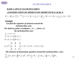
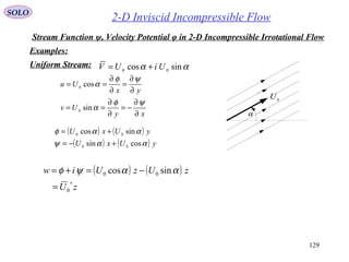
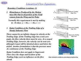
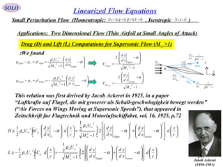
Small Perturbation Flow (Homentropic: , Isentropic )( )0~,0,0~,0 ==== τQqsd ( )0
=×∇ u
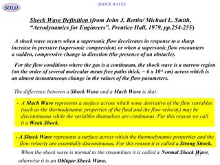
Applications: Two Dimensional Flow (Thin Airfoil at Small Angles of Attack)
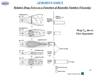
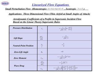
Several improved formulas where developed:
( )[ ] 2/11/1 0
0
222
p
p
p
CMMM
C
C
∞∞∞ −++−
= Karman-Tsien
Rule
Linearized Flow Equations
( ) 0
0
2222
12/
2
1
11 p
p
p
CMMMM
C
C
−
−
++−
=
∞∞∞∞
γ
Laitone’s
Rule
Comparison of several compressibility corrections
compared with experimental results for NACA 4412
Airfoil at an angle of attack of α = 1◦
.
Return to Table of Content](https://image.slidesharecdn.com/fluiddynamics-141022060736-conversion-gate02/85/Fluid-dynamics-238-320.jpg)
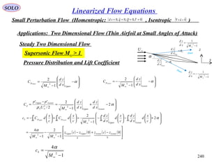
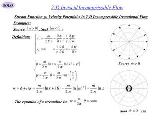
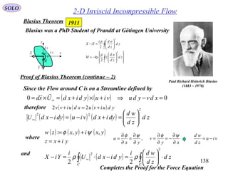
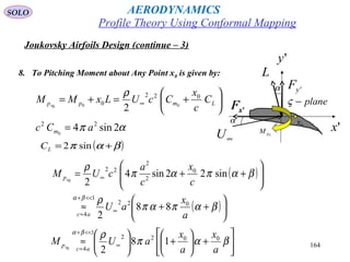
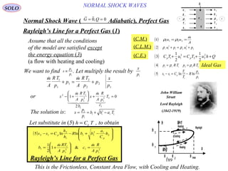
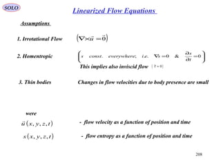
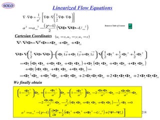
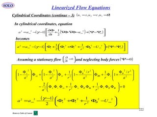
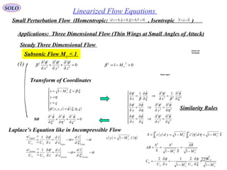
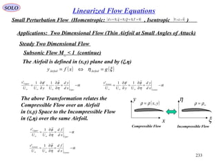
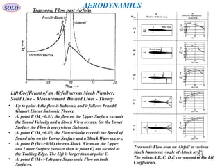
![247
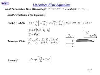
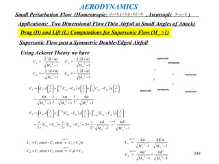
SOLO
Linearized Flow Equations
Small Perturbation Flow (Homentropic: , Isentropic )( )0~,0,0~,0 ==== τQqsd ( )0
=×∇ u
Applications: Two Dimensional Flow (Thin Airfoil at Small Angles of Attack)
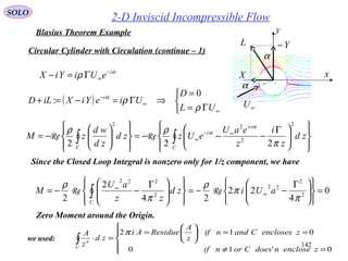
Steady Two Dimensional Flow
Supersonic Flow M∞ > 1
Pitching Moment Coefficient
The Pitching Moment Coefficient about the
Leading Edge for any Thin Airfoil is given by
xdx
xd
zd
xd
zd
Mcc
x
d
c
x
C
c
x
d
c
x
Cc
c
LowerUpper
ppM LowerUpperLE ∫∫∫
−+
−
−
−=
+
−=−
∞
022
1
0
1
0
1
2
αα
Thus
+
−
+
−
−= ∫∫
∞∞
xdzxdz
McM
c
c
Lower
c
UpperM LE 00222
1
2
1
2α
( ) ( ) ( ) ( )[ ] xdzxdzczczcxdzzxxdzzxxdx
xd
zd
xd
zd c
Lower
c
UpperLowerUpper
c
Lower
cx
xLower
c
Upper
cx
xUpper
c
LowerUpper
∫∫∫∫∫ −−−=−+−=
+
=
=
=
= 00
0
00000
Using integration by parts
Symmetric Airfoil zUpper = -zLower
1
2
2
−
−=
∞M
cM
α
The distance of the Airfoil Center of Pressure aft of the Leading Edge is given by
cc
M
M
c
c
c
c
x
L
MN
2
1
1/4
1/2
2
2
=⋅
−
−
=⋅−=
∞
∞
α
α
α
L
∞U
x
Return to Table of Content](https://image.slidesharecdn.com/fluiddynamics-141022060736-conversion-gate02/85/Fluid-dynamics-247-320.jpg)
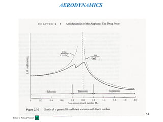
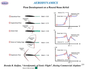


This document provides a table of contents for topics in fluid dynamics. It begins with mathematical notations for vectors, tensors, divergence, gradient, and other vector calculus topics. It then outlines the basic laws of fluid dynamics, such as conservation of mass and momentum. Later sections cover specific fluid dynamics concepts like boundary layers, compressible flow, shock waves, and potential flow. The document provides the framework for equations and analyses of fluid flows.