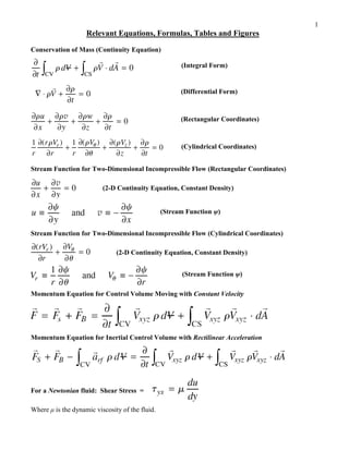
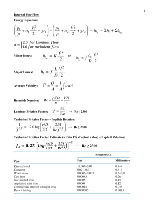
This document contains equations, formulas, tables and figures related to fluid mechanics. It includes the continuity equation, stream function, momentum equation, equations for shear stress, pressure variation in static fluids, fluid translation/deformation/rotation, the Bernoulli equation, equations for internal pipe flow including the energy equation, Reynolds number, friction factor, and equations for pumps/fans/blowers. It also includes properties tables for water and air, dimensional analysis concepts, and equations for similitude and dimensionless numbers including Reynolds, Weber, Cavitation, Euler, Froude and Mach numbers.

![10
DIMENSIONAL HOMOGENEITY AND DIMENSIONAL ANALYSIS
Equations that are in a form that do not depend on the fundamental units of measurement are called
dimensionally homogeneous equations. A special form of the dimensionally homogeneous equation is
one that involves only dimensionless groups of terms.
Buckingham’s Theorem: The number of independent dimensionless groups that may be employed to
describe a phenomenon known to involve n variables is equal to the number ( )
r
n − , where r is the
number of basic dimensions (i.e., M, L, T) needed to express the variables dimensionally.
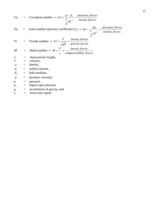
SIMILTUDE
In order to use a model to simulate the conditions of the prototype, the model must be geometrically,
kinematically, and dynamically similar to the prototype system.
To obtain dynamic similarity between two flow pictures, all independent force ratios that can be written
must be the same in both the model and the prototype. Thus, dynamic similarity between two flow
pictures (when all possible forces are acting) is expressed in the five simultaneous equations below.
[ ] [ ]
[ ] [ ]
[ ] [ ]
[ ] [ ]m
p
m
p
m
T
L
p
T
L
m
p
m
v
p
v
m
E
L
p
E
L
m
p
m
p
m
G
L
p
G
L
m
p
m
p
m
V
L
p
V
L
m
p
m
p
L
p
p
L
We
We
LV
LV
F
F
F
F
Ca
Ca
E
V
E
V
F
F
F
F
Fr
Fr
Lg
V
Lg
V
F
F
F
F
VL
VL
F
F
F
F
p
V
p
V
F
F
F
F
=
=
=
=
=
=
=
=
=
=
=
=
=
=
=
=
=
=
=
=
=
=
=
σ
ρ
σ
ρ
ρ
ρ
µ
ρ
µ
ρ
ρ
ρ
2
2
2
2
2
2
2
2
Re
Re
where the subscripts p and m stand for prototype and model respectively, and
L
F = inertia force → 2
2
L
V
ρ
P
F = pressure force → 2
L
p
A
p ∆
∝
∆
V
F = viscous force → VL
L
L
V
A
dy
du
A µ
µ
µ
τ =
∝
= 2
G
F = gravity force → 3
L
g
mg ρ
∝
E
F = elastic force → 2
L
E
A
E v
v ∝
T
F = surface tension force → L
σ
Re = Reynolds number →
forces
viscous
forces
inertia
v
VD
VD
=
=
=
µ
ρ
Re
We = Weber number →
forces
tension
surface
forces
inertia
L
V
We =
=
σ
ρ 2](https://image.slidesharecdn.com/fluidmechanicsbooklet-231104033822-80d0881f/85/FluidMechanicsBooklet-pdf-10-320.jpg)


![FLUID DYNAMICS [EQUATION OF MOTION].pptx](https://cdn.slidesharecdn.com/ss_thumbnails/fluiddynamicsequationofmotion-250628150614-29ccfaab-thumbnail.jpg?width=640&height=640&fit=bounds)


