This chapter discusses differential analysis of fluid flow. It introduces the concepts of stream function and vorticity. The key equations derived are:
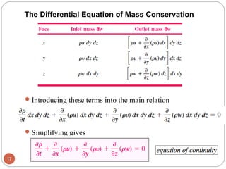
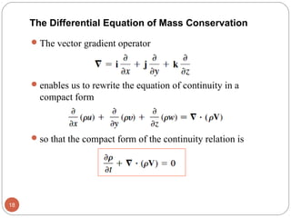
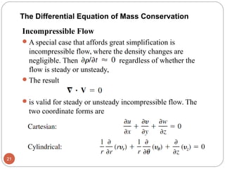
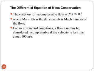
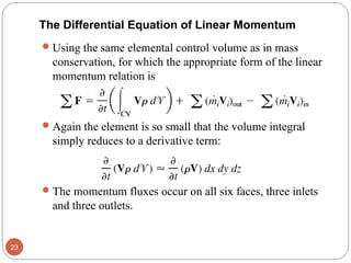
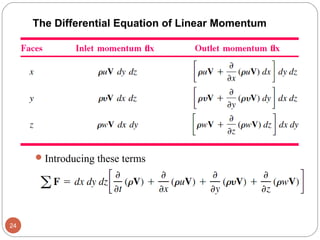
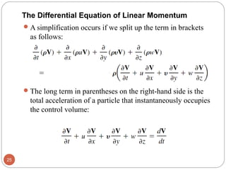
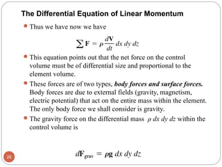
1) The differential equations of continuity, linear momentum, and mass conservation which relate the time rate of change of fluid properties like density and velocity within an infinitesimal control volume.
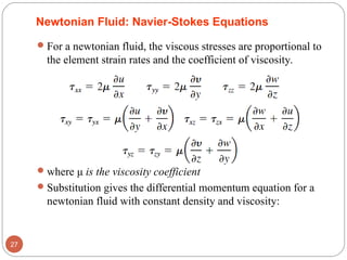
2) The Navier-Stokes equations which model viscous flow using Newton's laws and relate stresses to strain rates via viscosity.
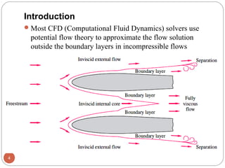
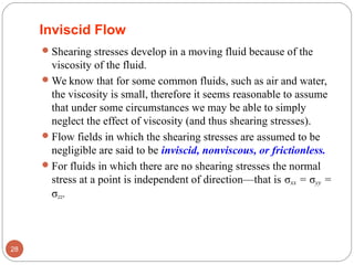
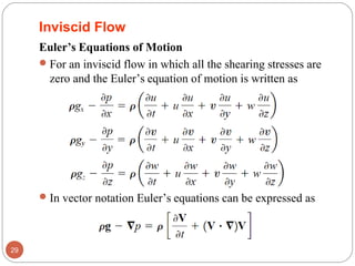
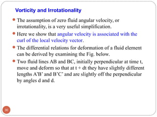
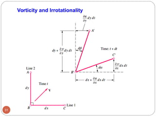
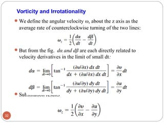
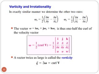
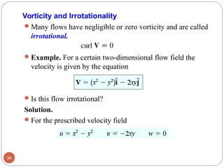
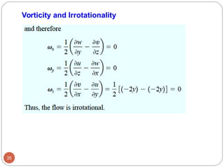
3) Equations for inviscid, irrotational flow where viscosity and vorticity are neglected.
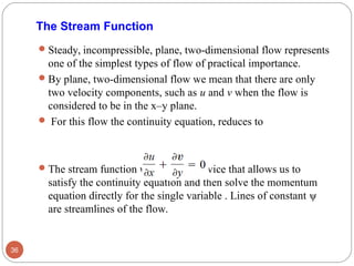
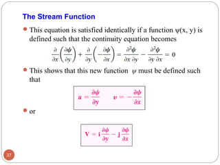
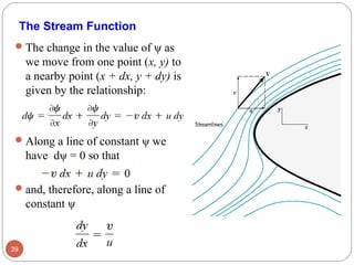
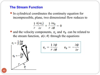
4) The stream function, a potential function whose contour lines represent streamlines, allowing 2D problems to be solved using a