Downloaded 83 times

![Therefore they represent a possible case of fluid flow. The rotation w of any fluid element in
the flow field is,
( ) ( )[ ] 0
2
1
2
33
2
2
1
2
1
2222
2
33
2
=−−−=
⎥
⎦
⎤
⎢
⎣
⎡
⎟⎟
⎠
⎞
⎜⎜
⎝
⎛
−+
∂
∂
−⎟⎟
⎠
⎞
⎜⎜
⎝
⎛
−−
∂
∂
=
⎟⎟
⎠
⎞
⎜⎜
⎝
⎛
∂
∂
−
∂
∂
=
xyxy
yxx
y
y
x
yxy
x
y
u
x
v
w
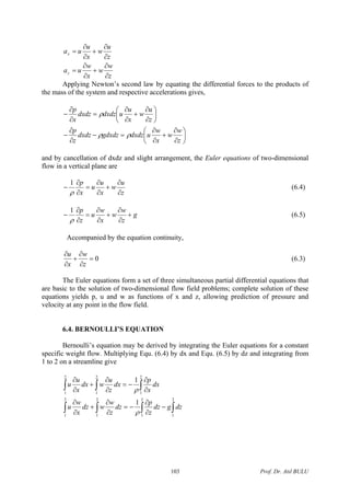
6.6. CIRCULATION AND VORTICITY
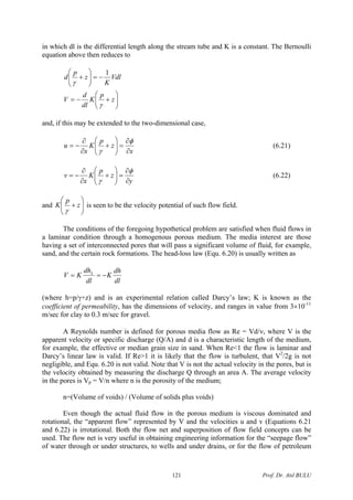
Consider a fluid element ABCD in rotational motion. Let the velocity components
along the sides of the element be as shown in Fig. 6.5.
u
yu + dy
Direction
of
intergration
u
vdy
dx
A D
CB
v + dx
v
x
y
x
Fig. 6.5
Since the element is rotating, being part of rotational flow, there must be a resultant
peripheral velocity. However, since the center of rotation is not known, it is more convenient
to relate rotation to the sum of products of velocity and distance around the contour of the
element. Such a sum is the line integral of velocity around the element and it is called
circulation, denoted by Γ. Thus,
∫ ⋅=Γ sdV
rr
(6.10)
Circulation is, by convention, regarded as positive for anticlockwise direction of
integration. Thus, for the element ABCD, from side AD
Prof. Dr. Atıl BULU107](https://image.slidesharecdn.com/chapter6-160123213822/85/TWO-DIMENSIONAL-IDEAL-FLOW-Chapter-6-8-320.jpg)
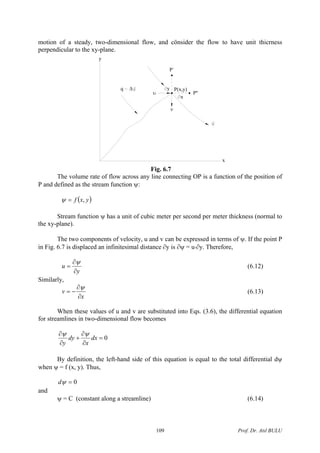
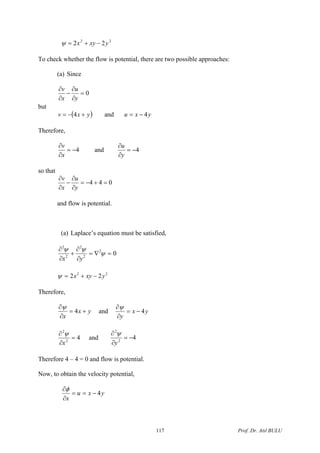


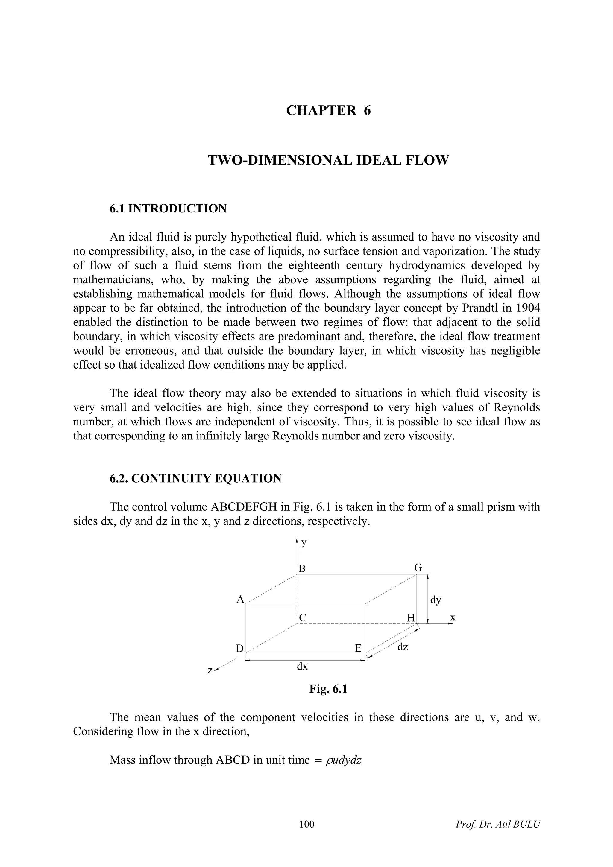
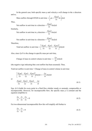
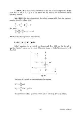
This document discusses two-dimensional ideal fluid flow. It begins by defining an ideal fluid as having no viscosity, compressibility, or surface tension. The continuity equation is then derived, stating that the net flow out of a control volume must equal the change in mass within the volume. Euler's equations are also derived, forming a set of partial differential equations that can be solved to determine pressure and velocity fields. Bernoulli's equation is obtained by integrating the Euler equations, relating total pressure, velocity, and elevation. The concepts of rotational and irrotational flow are introduced, with irrotational flow defined as having zero rotation of any fluid element.


