Download as PDF, PPTX

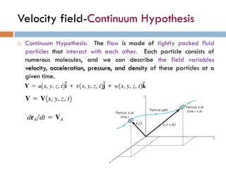
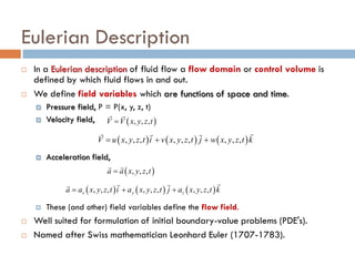
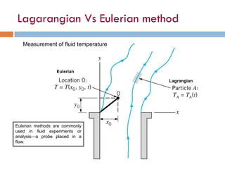

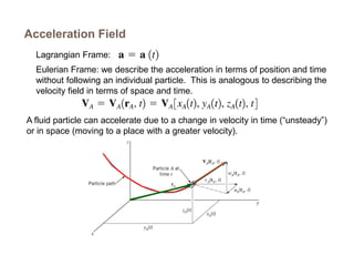
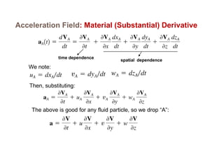
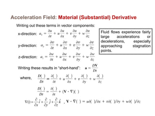
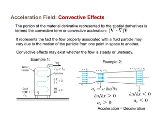
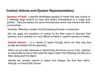
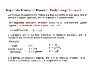
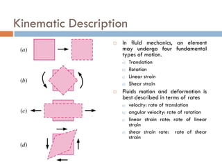

1) The document discusses fluid kinematics, which deals with the motion of fluids without considering the forces that create motion. It covers topics like velocity fields, acceleration fields, control volumes, and flow visualization techniques. 2) There are two main descriptions of fluid motion - Lagrangian, which follows individual particles, and Eulerian, which observes the flow at fixed points in space. Most practical analysis uses the Eulerian description. 3) The Reynolds Transport Theorem allows equations written for a fluid system to be applied to a fixed control volume, which is useful for analyzing forces on objects in a flow. It relates the time rate of change of an extensive property within the control volume to surface fluxes and the property accumulation.