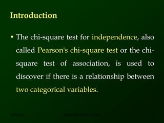
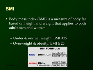
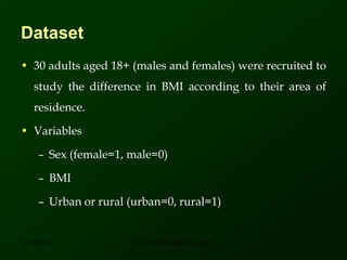
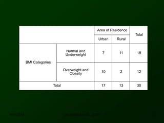
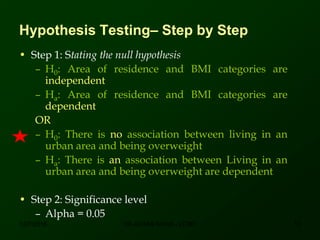
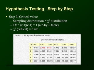
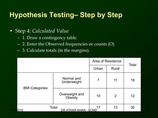
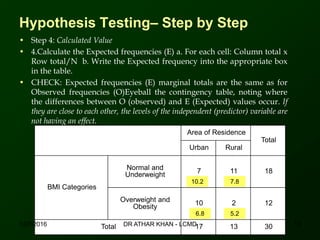
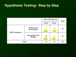
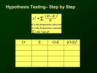
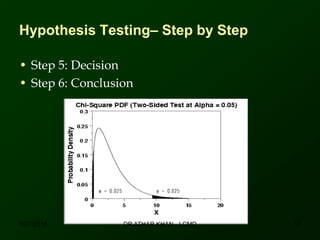
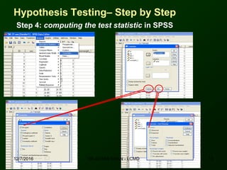
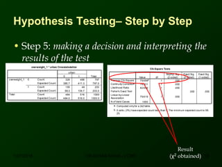
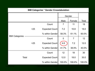
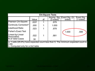
This document discusses using SPSS to conduct a chi-square test of independence. It provides an example of testing whether there is an association between area of residence (urban vs. rural) and BMI categories (normal weight vs. overweight/obese). The chi-square test involves stating hypotheses, calculating expected and observed frequencies, computing the test statistic in SPSS, and making a decision. No significant relationship was found between gender and BMI categories in another example exercise.

1. Using SPSS for Chi Square
Dr Athar Khan
MBBS, MCPS, DPH, DCPS-HCSM, DCPS-HPE, MBA,
PGD-Statistics
Associate Professor
Liaquat College of Medicine & Dentistry

2. Outline
• Introduction
• Dataset
• Chi-square
• Exercise
12/7/2016 2DR ATHAR KHAN - LCMD

3. Introduction
• The chi-square test for independence, also
called Pearson's chi-square test or the chi-
square test of association, is used to
discover if there is a relationship between
two categorical variables.
12/7/2016 3DR ATHAR KHAN - LCMD

4. BMI
• Body mass index (BMI) is a measure of body fat
based on height and weight that applies to both
adult men and women.
– Under & normal weight: BMI <25
– Overweight & obesity: BMI ≥ 25
12/7/2016 4DR ATHAR KHAN - LCMD

5. Question 1
• Is there any association between living in
a suburban area and being overweight?
– Under & normal weight: BMI <25
– Overweight & obese: BMI ≥ 25
Chi Square test
12/7/2016 5DR ATHAR KHAN - LCMD

6. Dataset
• 30 adults aged 18+ (males and females) were recruited to
study the difference in BMI according to their area of
residence.
• Variables
– Sex (female=1, male=0)
– BMI
– Urban or rural (urban=0, rural=1)
12/7/2016 6DR ATHAR KHAN - LCMD

7. Area of Residence
Total
Urban Rural
BMI Categories
Normal and
Underweight 7 11 18
Overweight and
Obesity 10 2 12
Total 17 13 30
12/7/2016 7DR ATHAR KHAN - LCMD

8. Assumptions
• Assumption #1:
• Two variables should be measured at
an ordinal or nominal
level (i.e., categorical data).
12/7/2016 8DR ATHAR KHAN - LCMD

9. Assumptions
• Assumption #2:
• Two variable should consist of two or more
categorical, independent groups. Example
independent variables that meet this criterion
include gender (2 groups: Males and Females),
ethnicity (e.g., 3 groups: Caucasian, African
American and Hispanic), physical activity level
(e.g., 4 groups: sedentary, low, moderate and
high), profession (e.g., 5 groups: surgeon, doctor,
nurse, dentist, therapist), and so forth.
12/7/2016 9DR ATHAR KHAN - LCMD

10. Hypothesis Testing– Step by Step
• Step 1: Stating the null hypothesis
– H0: Area of residence and BMI categories are
independent
– Ha: Area of residence and BMI categories are
dependent
OR
– H0: There is no association between living in an
urban area and being overweight
– Ha: There is an association between Living in an
urban area and being overweight are dependent
• Step 2: Significance level
– Alpha = 0.05
12/7/2016 10DR ATHAR KHAN - LCMD

11. Hypothesis Testing– Step by Step
• Step 3: Critical value
– Sampling distribution = χ2 distribution
– Df = (r-1)(c-1) = 1 (a 2-by-2 table)
– χ2 (critical) = 3.481
12/7/2016 11DR ATHAR KHAN - LCMD

12. Hypothesis Testing– Step by Step
• Step 4: Calculated Value
– 1. Draw a contingency table.
– 2. Enter the Observed frequencies or counts (O)
– 3. Calculate totals (in the margins).
Area of Residence
Total
Urban Rural
BMI Categories
Normal and
Underweight 7 11 18
Overweight and
Obesity 10 2 12
Total 17 13 30
12/7/2016 12DR ATHAR KHAN - LCMD

13. Hypothesis Testing– Step by Step
• Step 4: Calculated Value
• 4.Calculate the Expected frequencies (E) a. For each cell: Column total x
Row total/N b. Write the Expected frequency into the appropriate box
in the table.
• CHECK: Expected frequencies (E) marginal totals are the same as for
Observed frequencies (O)Eyeball the contingency table, noting where
the differences between O (observed) and E (Expected) values occur. If
they are close to each other, the levels of the independent (predictor) variable are
not having an effect.
Area of Residence
Total
Urban Rural
BMI Categories
Normal and
Underweight 7 11 18
Overweight and
Obesity 10 2 12
Total 17 13 30
10.2 7.8
6.8 5.2
12/7/2016 13DR ATHAR KHAN - LCMD

14. Important Point:
Chi-square can be used if no more than 20% of
the expected frequencies are less than 5 and none
is less than 1 (see note 'a.' at the bottom of SPSS
output to see if this is a problem).
It is possible to 'pool' or 'collapse' categories into
fewer, but this must only be done if it is meaningful
to group the data in this way.
12/7/2016 14DR ATHAR KHAN - LCMD

15. Hypothesis Testing– Step by Step
Area of Residence
Total
Urban Rural
BMI Categories
Normal and
Underweight 7 11 18
Overweight and
Obesity 10 2 12
Total 17 13 30
10.2 7.8
6.8 5.2
12/7/2016 15DR ATHAR KHAN - LCMD

16. Hypothesis Testing– Step by Step
O E O-E (O-E)2
12/7/2016 16DR ATHAR KHAN - LCMD

17. Hypothesis Testing– Step by Step
• Step 5: Decision
• Step 6: Conclusion
12/7/2016 17DR ATHAR KHAN - LCMD

18. Hypothesis Testing– Step by Step
Step 4: computing the test statistic in SPSS
12/7/2016 18DR ATHAR KHAN - LCMD

19. Hypothesis Testing– Step by Step
• Step 5: making a decision and interpreting the
results of the test
overweight_1 * urban Crosstabulation
329 468 797
385.7 411.3 797.0
155 48 203
98.3 104.7 203.0
484 516 1000
484.0 516.0 1000.0
Count
Expected Count
Count
Expected Count
Count
Expected Count
0
1
overweight_1
Total
0 1
urban
Total
Chi-Square Tests
79.699b 1 .000
78.301 1 .000
82.696 1 .000
.000 .000
79.619 1 .000
1000
Pearson Chi-Square
Continuity Correctiona
Likelihood Ratio
Fisher's Exact Test
Linear-by-Linear
Association
N of Valid Cases
Value df
Asymp. Sig.
(2-sided)
Exact Sig.
(2-sided)
Exact Sig.
(1-sided)
Computed onlyfor a 2x2 tablea.
0 cells (.0%) have expected count less than 5. The minimum expected count is 98.
25.
b.
Result
(χ2 obtained)12/7/2016 19DR ATHAR KHAN - LCMD

20. Exercise
• Does a significant relationship exist between
Gender and BMI categories ?
12/7/2016 20DR ATHAR KHAN - LCMD

21. BMI Categories * Gender Crosstabulation
Gender
TotalMale Female
BMI Categories
<25
Count 7 11 18
Expected Count 7.2 10.8 18.0
% within Gender 58.3% 61.1% 60.0%
>25
Count 5 7 12
Expected Count 4.8 7.2 12.0
% within Gender 41.7% 38.9% 40.0%
Total
Count 12 18 30
Expected Count 12.0 18.0 30.0
% within Gender 100.0% 100.0% 100.0%
12/7/2016 21DR ATHAR KHAN - LCMD

22. Chi-Square Tests
Value df
Asymp. Sig.
(2-sided)
Exact Sig. (2-
sided)
Exact Sig.
(1-sided)
Pearson Chi-Square .023a 1 .879
Continuity Correctionb
.000 1 1.000
Likelihood Ratio .023 1 .879
Fisher's Exact Test 1.000 .588
Linear-by-Linear
Association .022 1 .881
N of Valid Cases 30
a. 1 cells (25.0%) have expected count less than 5. The minimum expected count is
4.80.
b. Computed only for a 2x2 table
12/7/2016 22DR ATHAR KHAN - LCMD