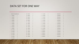
The document discusses the application of one-way and two-way ANOVA methods to analyze the effectiveness of three stress reduction treatments (medical, mental, and physical) on participants' stress levels, with considerations for gender as a blocking factor. It presents data analysis results that reject the assumptions of normality for treatment groups while not rejecting the equality of variances, leading to the use of non-parametric tests like the Kruskal-Wallis test. It concludes that there are significant differences in treatment effects and interactions between treatment and gender, warranting further analysis of treatment impacts by gender.

1. ONE WAY ANOVA
TWO WAY ANOVA
BY SEAN STOVALL

2. ONE WAY ANOVA

3. QUESTION POSED
• This dataset contains sample of 60 participants who are divided into three stress
reduction treatment groups (mental, physical, and medical). The stress reduction
values are represented on a scale that ranges from 1 to 5. This dataset can be
conceptualized as a comparison between three stress treatment programs, one
using mental methods, one using physical training, and one using medication.
The values represent how effective the treatment programs were at reducing
participant's stress levels, with higher numbers indicating higher effectiveness.

4. OBJECTIVE
• Compare the effect of Treatments (Medical, Mental, and Physical) on reducing
stress
• Let µ1, µ2, and µ3 be the following:
• µ1= true mean of stress reduction for the medical treatment group
• µ2= true mean of stress reduction for the mental treatment group
• µ3= true mean of stress reduction for the physical treatment group

5. DATA SET FOR ONE WAY
• Treatment StressReduction
• 1 medical 1
• 2 medical 1
• 3 medical 1
• 4 medical 1
• 5 medical 2
• 6 medical 2
• 7 medical 3
• 8 medical 3
• 9 medical 3
• 10 medical 3
• 11 medical 1
• 12 medical 1
• 13 medical 2
• 14 medical 2
• 15 medical 2
• 16 medical 2
• 17 medical 2
• 18 medical 2
• 19 medical 3
• 20 medical 3
• 21 mental 3
• 22 mental 3
• 23 mental 4
• 24 mental 4
• 25 mental 4
• 26 mental 4
• 27 mental 4
• 28 mental 4
• 29 mental 5
• 30 mental 5
• 31 mental 2
• 32 mental 2
• 33 mental 2
• 34 mental 2
• 35 mental 3
• 36 mental 3
• 37 mental 4
• 38 mental 4
• 39 mental 4
• 40 mental 4
• 41 physical 1
• 42 physical 1
• 43 physical 1
• 44 physical 1
• 45 physical 2
• 46 physical 2
• 47 physical 3
• 48 physical 3
• 49 physical 3
• 50 physical 3
• 51 physical 3
• 52 physical 3
• 53 physical 4
• 54 physical 4
• 55 physical 4
• 56 physical 4
• 57 physical 4
• 58 physical 4
• 59 physical 5
• 60 physical 5

6. HYPOTHESES
• Hypothesis of interest
• H0: mean of stress reduction does not differ among treatment groups
• µ1=µ2=µ3
• µ1-Medical, µ2-Mental, µ3-Physical
•
• H1: mean of stress reduction differs among treatment groups, at least one pair not equal. (µi, µj) are not equal i≠j
• µ1= µ2
• µ1= µ3
• µ2= µ3

7. ASSUMPTIONS
• #1) All 3 treatments should follow independent normal distribution
• #2) The equality of variances for all 3 treatments
• H0: σ1= σ2= σ3
• H1: At least one pair is not equal

8. TESTING FOR ASSUMPTION 1
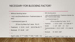
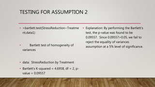
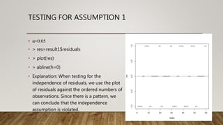
• >tapply(data$StressRed
uction,data$Treatment,s
hapiro.test)
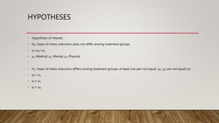
• $medical
• Shapiro-Wilk
normality test
• data: X[[i]]
• W = 0.81255, p-value =
0.001337
• $mental
• Shapiro-Wilk
normality test
• data: X[[i]]
• W = 0.84416, p-value
= 0.004262
• $physical
• Shapiro-Wilk
normality test
• data: X[[i]]
• W = 0.8943, p-value =
0.03228

9. EXPLANATION
• Medical: From the shapiro test, the medical treatment group’s p-value was found to
be 0.001337. Since 0.00137<0.05, we reject the normality assumption at a 5% level of
significance.
• Mental: From the shapiro test, the mental treatment group’s p-value was found to be
0.004262. Since 0.004262<0.05, we reject the normality assumption at a 5% level of
significance.
• Physical: From the shapiro test, the physical treatment group’s p-value was found to
be 0.03228. Since 0.03228<0.05, we reject the normality assumption at a 5% level of
significance.
• Overall conclusion: Since for all 3 levels of treatment we reject the normality
assumption, we can conclude the normality assumption fails for all 3 levels at a 5%
level of significance.

10. TESTING FOR ASSUMPTION 2
• >bartlett.test(StressReduction~Treatme
nt,data1)
• Bartlett test of homogeneity of
variances
• data: StressReduction by Treatment
• Bartlett's K-squared = 4.6958, df = 2, p-
value = 0.09557
• Explanation: By performing the Bartlett’s
test, the p-value was found to be
0.09557. Since 0.09557>0.05, we fail to
reject the equality of variances
assumption at a 5% level of significance.

11. RESULTS FROM ASSUMPTIONS
• From the assumptions, the normality assumption was rejected for all 3 treatment
groups, but the equal variances assumption was not rejected. The equality of
means now must be tested and if that is rejected, then we must carry out another
test to find which pair led to the rejection of H0. Since the first assumption was
rejected, we must carry out a non-parametric setup such as Kruskal Wallis test to
test for the equality of means.

12. TESTING FOR EQUALITY OF MEANS
• >kruskal.test(StressReduction~Treatme
nt,data1)
• Kruskal-Wallis rank sum test
• data: StressReduction by Treatment
• Kruskal-Wallis chi-squared = 16.993, df
= 2, p-value = 0.0002041
• Explanation: The p-value found from
the Kruskal.test was found to be
0.0002041. Since 0.0002041<0.05, we
reject the null hypothesis and cannot
consider the different treatment
means to be equal. This means that
the treatments have different effects
and are effective at a 5% level of
significance.
• The next step for this would be to
find which pair of means actually led
to the rejection of H0.

13. KRUSKAL WALLIS NON-PARAMETRIC
• >kruskalmc(data1$StressReduction,data1$
Treatment,probs=0.05)
• Multiple comparison test after Kruskal-
Wallis
• p.value: 0.05
• Comparisons
• obs.dif critical.dif difference
• medical-mental 21.7 13.22119
TRUE
• medical-physical 14.6 13.22119
TRUE
• mental-physical 7.1 13.22119
• Explanation: From the Kruskal
Wallis test, the mean groups
medical-mental and medical-
physical say “True”. This means
that here is a difference between
the two pairs and is what led to the
rejection of H0:µ1=µ2=µ3.
•

14. BRING IN BLOCKING
FACTOR

15. TWO WAY ANOVA

16. QUESTION POSED
• This dataset contains sample of 60 participants who are divided into three stress
reduction treatment groups (mental, physical, and medical) and two gender
groups (male and female). The stress reduction values are represented on a scale
that ranges from 1 to 5. This dataset can be conceptualized as a comparison
between three stress treatment programs, one using mental methods, one using
physical training, and one using medication across genders. The values represent
how effective the treatment programs were at reducing participant's stress levels,
with higher numbers indicating higher effectiveness.

17. OBJECTIVE
• Compare the effect of Treatments (Medical, Mental, and Physical) on reducing
stress with the additional effect of gender.
• Groups: Treatments (Medical, Mental, and Physical)
• Blocks: Gender (Male, Female)

18. DATA SET FOR TWO WAY
• Treatment Gender StressReduction
• 1 medical F 1
• 2 medical F 1
• 3 medical F 1
• 4 medical F 1
• 5 medical F 2
• 6 medical F 2
• 7 medical F 3
• 8 medical F 3
• 9 medical F 3
• 10 medical F 3
• 11 medical M 1
• 12 medical M 1
• 13 medical M 2
• 14 medical M 2
• 15 medical M 2
• 16 medical M 2
• 17 medical M 2
• 18 medical M 2
• 19 medical M 3
• 20 medical M 3
• 21 mental F 3
• 22 mental F 3
• 23 mental F 4
• 24 mental F 4
• 25 mental F 4
• 26 mental F 4
• 27 mental F 4
• 28 mental F 4
• 29 mental F 5
• 30 mental F 5
• 31 mental M 2
• 32 mental M 2
• 33 mental M 2
• 34 mental M 2
• 35 mental M 3
• 36 mental M 3
• 37 mental M 4
• 38 mental M 4
• 39 mental M 4
• 40 mental M 4
• 41 physical F 1
• 42 physical F 1
• 43 physical F 1
• 44 physical F 1
• 45 physical F 2
• 46 physical F 2
• 47 physical F 3
• 48 physical F 3
• 49 physical F 3
• 50 physical F 3
• 51 physical M 3
• 52 physical M 3
• 53 physical M 4
• 54 physical M 4
• 55 physical M 4
• 56 physical M 4
• 57 physical M 4
• 58 physical M 4
• 59 physical M 5
• 60 physical M 5

19. NULL HYPOTHESES
• H01: (treatments) Equality of means for different groups of interest.
• µ1=µ2=µ3
• µ1-Medical, µ2-Mental, µ3-Physical
• where i≠g
• H02: (Gender) No mean difference among different levels of the block.
• Γ1= Γ2
• Γ1-Male, Γ2-Female
• H03: No interaction between the Groups and Blocks.
• Groups- Treatments (Medical, Mental, Physical)
• Blocks- Genders (Male, Female)

20. ALTERNATIVE HYPOTHESES
• H1: At least one pair of mean treatments is not equal
• Pairs possible:
• µ1= µ2
• µ1= µ3
• µ2= µ3
• H2: There is a mean difference between genders
• Pairs possible:
• Male=Female
• H3: There is an interaction between Groups and Blocks
• Groups- Treatments (Medical, Mental, Physical)
• Blocks- Genders (Male, Female)

21. ASSUMPTIONS
• # 1) Observations corresponding to each cell should follow independent normal
distribution
• # 2) Observations corresponding to each cell should have equal variances
• α=0.05

22. BALANCED DATA SET
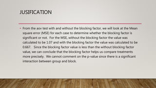
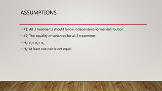
• Explanation: The observations
corresponding to each level of
treatment and gender are the
same, so the corresponding design/
layout is balanced. Or by looking
at the data, there are 60 samples, 3
levels of treatment, and 2 genders.
The 6 combinations would be as
follows: M/med, M/ment, M/phys,
F/med, F/ment, and F/phys
• 60/6=10
• > # check for balance or unbalanced
• >
nrow(data[data$Gender=="M"&data$Treatment=="medical",
])
• [1] 10
• >
nrow(data[data$Gender=="M"&data$Treatment=="mental",]
)
• [1] 10
• >
nrow(data[data$Gender=="M"&data$Treatment=="physical",
])
• [1] 10
• >
nrow(data[data$Gender=="F"&data$Treatment=="medical",]
)
• [1] 10
• >
nrow(data[data$Gender=="F"&data$Treatment=="mental",])
• [1] 10

23. TESTING FOR ASSUMPTION 1
• α=0.05
• > res=result1$residuals
• > plot(res)
• > abline(h=0)
• Explanation: When testing for the
independence of residuals, we use the plot
of residuals against the ordered numbers of
observations. Since there is a pattern, we
can conclude that the independence
assumption is violated.

24. TESTING FOR ASSUMPTION 2
• α=0.05
• > fit=result1$fitted.values
• > res=result1$residuals
• > plot(fit,res)
• > abline(h=0)
• Explanation: The plot of
residuals against fitted values is
not randomly scattered about
the horizontal line at 0. So the
conclusion is that the
assumption of equal variances
is violated.

25. ASSUMPTION VIOLATION
• Both assumptions are violated, but in this case will be taking the design of
experiment approach.

26. TRENDS GRAPHICALLY
• >plot(StressReduction~Gender+Treat
ment,data)
• Explanation: From the first boxplot
(left), we can say that the mean stress
reduction reported for the Gender (F
and M) appear to be similar. The
second boxplot (right), we can say that
the mean stress reduction for the
medical treatment, mental treatment
and physical treatment appear to be
significantly different. Mental
treatment mean was the highest
followed by physical treatment, and
the lowest was medical treatment.

27. INTERACTIONS GRAPHICALLY
• > par(mfrow=c(1,2))
• >interaction.plot(data$Treatment,
data$Gender,data$StressReductio
n)
• >interaction.plot(data$Gender,dat
a$Treatment,data$StressReductio
n)
• Explanation: From this interaction
plots (left and right), the lines
cross in both. Thus, we can
conclude there is a sign of
interaction between groups and
blocks (treatment and gender)
and cannot test the two
independently.

28. FORMAL INTERACTION TEST
• α=0.05
• >result1=aov(StressReduction~Treatment+Gender+Treatment
*Gender,data)
• > summary(result1)
• Df Sum Sq Mean Sq F value Pr(>F)
• Treatment 2 23.33 11.667 17.5 1.38e-06 ***
• Gender 1 1.67 1.667 2.5 0.12
• Treatment:Gender 2 23.33 11.667 17.5 1.38e-06 ***
• Residuals 54 36.00 0.667
• ---
• Signif. codes: 0 ‘***’ 0.001 ‘**’ 0.01 ‘*’ 0.05 ‘.’ 0.1 ‘ ’ 1
• Explanation: The aov test was used to test for the
interaction between group (Treatment) and block
(Gender) by looking at the p-value corresponding to
Treatment:Gender. From this test, a p-value of
1.384e-6 was found and compared to α=0.05. Since
1.384e-6<0.05, we reject the hypothesis of no
interaction (H03) at a 5% level of significance. From
this, we can conclude that there is a significant
interaction between treatment and gender, and we
cannot carry out independent tests for the main
effects.
• Next, it is recommended we carry out a one-way
ANOVA for each level of gender to see the impact on
treatments.
• This conclusion aligns with the interaction plot.

29. DIVIDE DATA
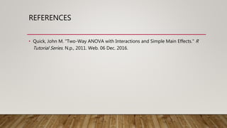
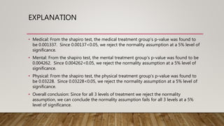
• > # Divide up the dataset based on gender
• > dataM=data[data$Gender=="M",]
• > dataF=data[data$Gender=="F",]

30. TREATMENT IMPACT ON MALE GENDER
• α=0.05>
aovM=aov(StressReduction~Treatment,dataM)
• > summary(aovM)
• Df Sum Sq Mean Sq F value Pr(>F)
• Treatment 2 20 10.000 16.88 1.76e-05 ***
• Residuals 27 16 0.593
• ---
• Signif. codes: 0 ‘***’ 0.001 ‘**’ 0.01 ‘*’ 0.05 ‘.’
0.1 ‘ ’ 1
• Explanation: The aov test was used to
test for the equality of treatments mean
for the male gender. From this test, a p-
value of 1.76e-5 was found and
compared to α=0.05. Since 1.76e-
5<0.05, we reject the equality of
treatment means and can conclude that
the treatments have an impact on the
male gender at a 5% level of
significance.
• The next step is to find which treatment
means are different and led to the
rejection of H0.

31. FIND WHICH TREATMENT
• > TukeyHSD(aovM,"Treatment",conf.level=0.95)
• Tukey multiple comparisons of means
• 95% family-wise confidence level
• Fit: aov(formula = StressReduction ~ Treatment, data =
dataM)
• $Treatment
• diff lwr upr p adj
• mental-medical 1 0.1464228 1.853577 0.0192139
• physical-medical 2 1.1464228 2.853577 0.0000102
• physical-mental 1 0.1464228 1.853577 0.0192139
• Explanation: From the Tukey’s test, the 95%
C.I. for all the mean treatment groups do not
include 0. We can conclude that all the
treatment means for the male gender are
different from each other and are what led
to the rejection of H0.

32. TREATMENT IMPACT ON FEMALE GENDER
• α=0.05
• >
aovF=aov(StressReduction~Treatment,data
F)
• > summary(aovF)
• Df Sum Sq Mean Sq F value Pr(>F)
• Treatment 2 26.67 13.333 18 1.08e-05
***
• Residuals 27 20.00 0.741
• ---
• Signif. codes: 0 ‘***’ 0.001 ‘**’ 0.01 ‘*’ 0.05 ‘.’
0.1 ‘ ’ 1
• Explanation: The aov test was used to
test for the equality of treatments
mean for the female gender. From
this test, a p-value of 1.08e-5 was
found and compared to α=0.05. Since
1.08e-5<0.05, we reject the equality of
treatment means and can conclude
that the treatments have an impact on
the female gender at a 5% level of
significance.
• The next step is to find which
treatment means are different and led
to the rejection of H0.

33. FIND WHICH TREATMENT
• > TukeyHSD(aovF,"Treatment",conf.level=0.95)
• Tukey multiple comparisons of means
• 95% family-wise confidence level
• Fit: aov(formula = StressReduction ~ Treatment, data =
dataF)
• $Treatment
• diff lwr upr p adj
• mental-medical 2 1.0456717 2.9543283 5.21e-05
• physical-medical 0 -0.9543283 0.9543283 1.00e+00
• physical-mental -2 -2.9543283 -1.0456717 5.21e-05
• Explanation: Explanation: From the Tukey’s
test, the 95% C.I. for the mean treatment
groups mental-medical and physical-metal do
not include 0. We can conclude that these
treatment means for the female gender are
different from each other and are what led to
the rejection of H0.

34. NECESSARY FOR BLOCKING FACTOR?
• Without blocking factor
• >res1=aov(StressReduction~Treatment,data=d
ata1)
• > summary(res1,type=3)
• Df Sum Sq Mean Sq F value Pr(>F)
• Treatment 2 23.33 11.67 10.9 9.79e-05 ***
• Residuals 57 61.00 1.07
• ---
• Signif. codes: 0 ‘***’ 0.001 ‘**’ 0.01 ‘*’ 0.05 ‘.’ 0.1
‘ ’ 1
• With blocking factor
• >res2=aov(StressReduction~Treatment+Gender+Ge
nder*Treatment,data=data)
• > summary(res2,type=3)
• Df Sum Sq Mean Sq F value Pr(>F)
• Treatment 2 23.33 11.667 17.5 1.38e-06 ***
• Gender 1 1.67 1.667 2.5 0.12
• Treatment:Gender 2 23.33 11.667 17.5 1.38e-06
***
• Residuals 54 36.00 0.667
• ---
• Signif. codes: 0 ‘***’ 0.001 ‘**’ 0.01 ‘*’ 0.05 ‘.’ 0.1 ‘ ’ 1

35. JUSIFICATION
• From the aov test with and without the blocking factor, we will look at the Mean
square error (MSE) for each case to determine whether the blocking factor is
significant or not. For the MSE, without the blocking factor the value was
calculated to be 1.07 and with the blocking factor the value was calculated to be
0.667. Since the blocking factor value is less than the without blocking factor
value, we can conclude that the blocking factor helps us compare treatments
more precisely. We cannot comment on the p-value since there is a significant
interaction between group and block.

36. REFERENCES
• Quick, John M. "Two-Way ANOVA with Interactions and Simple Main Effects." R
Tutorial Series. N.p., 2011. Web. 06 Dec. 2016.

37. QUESTIONS