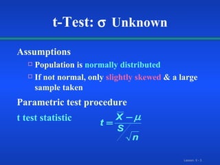
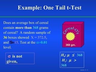
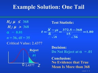
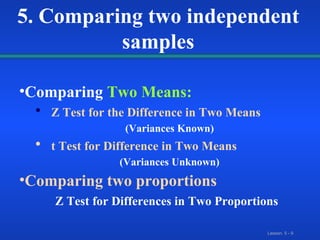
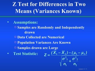
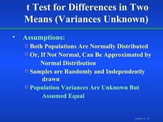
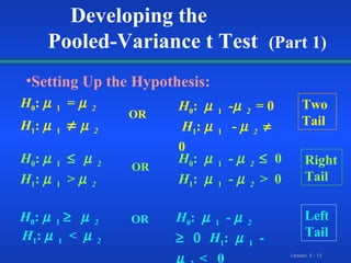
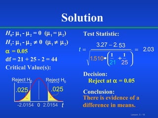
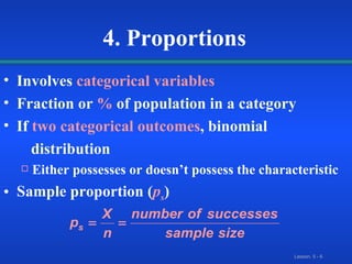
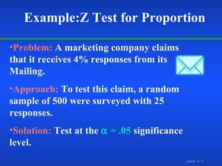
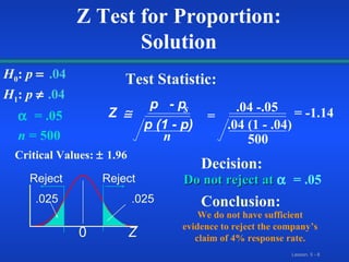
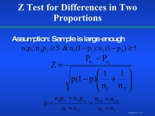
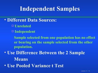
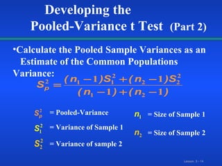
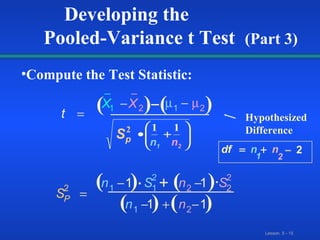
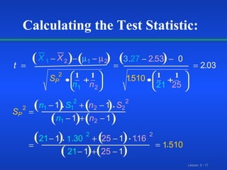
This document provides an overview of common statistical hypothesis tests, including: 1. One-tail and two-tail t-tests of hypotheses for the mean to compare a sample mean to a hypothesized population mean or compare two independent sample means. 2. Z-tests of hypotheses for a proportion to test a claim about a population proportion or compare two independent proportions. 3. Pooled variance t-tests to compare two independent sample means when population variances are unknown but assumed equal. Worked examples are provided to demonstrate how to set up the null and alternative hypotheses, calculate test statistics, determine critical values, and make decisions to reject or fail to reject the null hypothesis.

1. Statistics for Management Fundamentals of Hypothesis Testing

2. Lesson Topics 3. One Tail Test t Test of Hypothesis for the Mean 4. Proportions Z Test of Hypothesis for the Proportion 5. Comparing two independent samples

3. Assumptions Population is normally distributed If not normal, only slightly skewed & a large sample taken Parametric test procedure t test statistic t-Test:  Unknown

4. Example: One Tail t-Test Does an average box of cereal contain more than 368 grams of cereal? A random sample of 36 boxes showed X = 372.5 , and  S= 15 . Test at the  0.01 level. 368 gm. H 0 :   368 H 1 :  368  is not given,

5.  = 0.01 n = 36, df = 35 Critical Value: 2.4377 Test Statistic: Decision: Conclusion: Do Not Reject at  = .01 No Evidence that True Mean Is More than 368 Z 0 2.4377 .01 Reject Example Solution: One Tail H 0 :  368 H 1 :  368

6. Involves categorical variables Fraction or % of population in a category If two categorical outcomes , binomial distribution Either possesses or doesn’t possess the characteristic Sample proportion ( p s ) 4. Proportions

7. Example:Z Test for Proportion Problem: A marketing company claims that it receives 4% responses from its Mailing. Approach: To test this claim, a random sample of 500 were surveyed with 25 responses. Solution: Test at the  = .05 significance level.

8.  = .05 n = 500 Do not reject at  = .05 Z Test for Proportion: Solution H 0 : p  .04 H 1 : p  .04 Critical Values:  1.96 Test Statistic: Decision: Conclusion: We do not have sufficient evidence to reject the company’s claim of 4% response rate. Z  p - p p (1 - p) n s = .04 -.05 .04 (1 - .04) 500 = -1.14 Z 0 Reject Reject .025 .025

9. 5. Comparing two independent samples Comparing Two Means: Z Test for the Difference in Two Means (Variances Known) t Test for Difference in Two Means (Variances Unknown) Comparing two proportions Z Test for Differences in Two Proportions

10. Different Data Sources: Unrelated Independent Sample selected from one population has no effect or bearing on the sample selected from the other population. Use Difference Between the 2 Sample Means Use Pooled Variance t Test Independent Samples

11. Assumptions: Samples are Randomly and Independently drawn Data Collected are Numerical Population Variances Are Known Samples drawn are Large Test Statistic: Z Test for Differences in Two Means (Variances Known)

12. Assumptions: Both Populations Are Normally Distributed Or, If Not Normal, Can Be Approximated by Normal Distribution Samples are Randomly and Independently drawn Population Variances Are Unknown But Assumed Equal t Test for Differences in Two Means (Variances Unknown)

13. Developing the Pooled-Variance t Test (Part 1) Setting Up the Hypothesis: H 0 :  1   2 H 1 :  1 >  2 H 0 :  1 -  2 = 0 H 1 :  1 -  2  0 H 0 :  1 =  2 H 1 :  1   2 H 0 :  1   2  H 0 :  1 -  2  0 H 1 :  1 -  2 > 0 H 0 :  1 -  2  H 1 :  1 -  2 < 0 OR OR OR Left Tail Right Tail Two Tail  H 1 :  1 <  2

14. Developing the Pooled-Variance t Test (Part 2) Calculate the Pooled Sample Variances as an Estimate of the Common Populations Variance: = Pooled-Variance = Variance of Sample 1 = Variance of sample 2 = Size of Sample 1 = Size of Sample 2

15. t X X S n S n S n n df n n P                 1 2 1 2 2 1 1 2 2 2 2 1 2 1 2 1 1 1 1 2   Hypothesized Difference Developing the Pooled-Variance t Test (Part 3) Compute the Test Statistic: ( ) ) ( ( ) ( ) ( ) ( ) n 1 n 2 _ _

16. You’re a financial analyst for Charles Schwab. Is there a difference in dividend yield between stocks listed on the NYSE & NASDAQ? You collect the following data: NYSE NASDAQ Number 21 25 Mean 3.27 2.53 Std Dev 1.30 1.16 Assuming equal variances, is there a difference in average yield (  = 0.05 )? © 1984-1994 T/Maker Co. Pooled-Variance t Test: Example

17. t X X S n n S n S n S n n P P                            1 2 1 2 2 1 2 2 1 1 2 2 2 2 1 2 2 2 3 27 2 53 0 1 510 21 25 2 03 1 1 1 1 21 1 1 30 25 1 1 16 21 1 25 1 1 510   . . . . . . . Calculating the Test Statistic: ( ( ( ( ( ( ( ( ( ( ( ) ) ) ) ) ) ) ) ) ) )

18. H 0 :  1 -  2 = 0 (  1 =  2 ) H 1 :  1 -  2  0 (  1   2 )  = 0.05 df = 21 + 25 - 2 = 44 Critical Value(s): Test Statistic: Decision: Conclusion: Reject at  = 0.05 There is evidence of a difference in means. t 0 2.0154 -2.0154 .025 Reject H 0 Reject H 0 .025 t    3 27 2 53 1 510 21 25 2 03 . . . . Solution

19. Z Test for Differences in Two Proportions Assumption: Sample is large enough

20. Lesson Summary Made Connection to Confidence Interval Estimation Performed One Tail and Two Tail Tests Performed t Test of Hypothesis for the Mean Performed Z Test of Hypothesis for the Proportion Comparing two independent samples