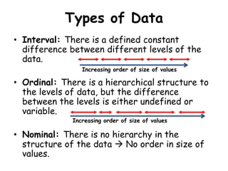
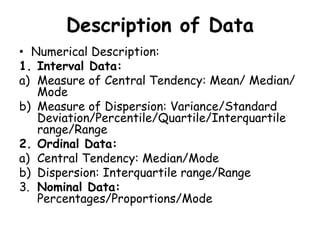
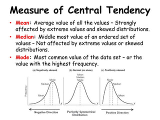
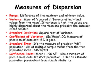
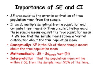
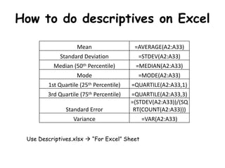
Types of Variables
and
Descriptive statistics
Dhritiman Chakrabarti
Assistant Professor,
Dept of Neuroanaesthesiology
and Neurocritical Care,
NIMHANS, Bangalore
Types of Data
• Interval: There is a defined constant
difference between different levels of the
data.
• Ordinal: There is a hierarchical structure to
the levels of data, but the difference
between the levels is either undefined or
variable.
• Nominal: There is no hierarchy in the
structure of the data  No order in size of
values.
Increasing order of size of values
Description of Data
• Numerical Description:
1. Interval Data:
a) Measure of Central Tendency: Mean/ Median/
Mode
b) Measure of Dispersion: Variance/Standard
Deviation/Percentile/Quartile/Interquartile
range/Range
2. Ordinal Data:
a) Central Tendency: Median/Mode
b) Dispersion: Interquartile range/Range
3. Nominal Data:
Percentages/Proportions/Mode
Measure of Central Tendency
• Mean: Average value of all the values – Strongly
affected by extreme values and skewed distributions.
• Median: Middle most value of an ordered set of
values – Not affected by extreme values or skewed
distributions.
• Mode: Most common value of the data set – or the
value with the highest frequency.
Measures of Dispersion
• Range: Difference of the maximum and minimum value.
• Variance: Mean of “squared difference of individual
values from the mean”. If variance is high, the values are
highly dispersed about the mean and probably the data set
is not reliable.
• Standard Deviation: Square root of Variance.
• Coefficient of Variation: SD/Mean*100; Measure of
precision of data set; <5% is good.
• Standard Error: It’s the measure of precision WRT
population – SD of multiple sample means from the true
population mean – SD/sqrtN.
• Confidence limits: Mean ± 1.96 SE – Also a measure of
precision of data set WRT population – Used to estimate
population parameters from sample statistics.
Importance of SE and CI
• SE encapsulates the error in estimation of true
population mean from the sample.
• If we do multiple samplings from a population and
compute their means  Then create a histogram of
these sample means against the true population mean
 We see that the sample means follow a Normal
distribution about the true population mean.
• Conceptually: SE is the SD of these sample means
about the true population mean.
• Mathematically: SE = Sdsample /sqrt(N)
• Interpretation: That the population mean will lie
within 2 SE from the sample mean 95% of the time.
How to do descriptives on Excel
Mean =AVERAGE(A2:A33)
Standard Deviation =STDEV(A2:A33)
Median (50th Percentile) =MEDIAN(A2:A33)
Mode =MODE(A2:A33)
1st Quartile (25th Percentile) =QUARTILE(A2:A33,1)
3rd Quartile (75th Percentile) =QUARTILE(A2:A33,3)
Standard Error
=(STDEV(A2:A33))/(SQ
RT(COUNT(A2:A33)))
Variance =VAR(A2:A33)
Use Descriptives.xlsx  “For Excel” Sheet
Descriptives in SPSS
• Import data into SPSS.
• Go to Analyze  Descriptive Statistics  Frequencies.
• Insert all Interval scale variables into the “Variables” box.
• Click on “Statistics” tab  Check all statistics that you want 
At minimum check mean, median, quartiles and stdev  Continue
• Uncheck “Display frequency tables”- Not required  Click OK
Output
SPSS Syntax - Ignore
Main Output – Self explanatory
Export to Excel for Tables
• Copy the output from SPSS output viewer.
• Open blank Excel sheet, Click on B2 cell and Paste.
Making tables using Concatenate
• Concatenate function helps to group
different cells of Excel into one.
• Just dragging the formula creates similar format - median
(IQR) for all variables  Makes making tables much easier.
• Next copy all the concatenates and “Paste Values”.
• Then copy and paste however you want on Word to make tables

Types of variables and descriptive statistics

  • 1.
    Types of Variables and Descriptivestatistics Dhritiman Chakrabarti Assistant Professor, Dept of Neuroanaesthesiology and Neurocritical Care, NIMHANS, Bangalore
  • 2.
    Types of Data •Interval: There is a defined constant difference between different levels of the data. • Ordinal: There is a hierarchical structure to the levels of data, but the difference between the levels is either undefined or variable. • Nominal: There is no hierarchy in the structure of the data  No order in size of values. Increasing order of size of values Increasing order of size of values
  • 3.
    Description of Data •Numerical Description: 1. Interval Data: a) Measure of Central Tendency: Mean/ Median/ Mode b) Measure of Dispersion: Variance/Standard Deviation/Percentile/Quartile/Interquartile range/Range 2. Ordinal Data: a) Central Tendency: Median/Mode b) Dispersion: Interquartile range/Range 3. Nominal Data: Percentages/Proportions/Mode
  • 4.
    Measure of CentralTendency • Mean: Average value of all the values – Strongly affected by extreme values and skewed distributions. • Median: Middle most value of an ordered set of values – Not affected by extreme values or skewed distributions. • Mode: Most common value of the data set – or the value with the highest frequency.
  • 5.
    Measures of Dispersion •Range: Difference of the maximum and minimum value. • Variance: Mean of “squared difference of individual values from the mean”. If variance is high, the values are highly dispersed about the mean and probably the data set is not reliable. • Standard Deviation: Square root of Variance. • Coefficient of Variation: SD/Mean*100; Measure of precision of data set; <5% is good. • Standard Error: It’s the measure of precision WRT population – SD of multiple sample means from the true population mean – SD/sqrtN. • Confidence limits: Mean ± 1.96 SE – Also a measure of precision of data set WRT population – Used to estimate population parameters from sample statistics.
  • 6.
    Importance of SEand CI • SE encapsulates the error in estimation of true population mean from the sample. • If we do multiple samplings from a population and compute their means  Then create a histogram of these sample means against the true population mean  We see that the sample means follow a Normal distribution about the true population mean. • Conceptually: SE is the SD of these sample means about the true population mean. • Mathematically: SE = Sdsample /sqrt(N) • Interpretation: That the population mean will lie within 2 SE from the sample mean 95% of the time.
  • 7.
    How to dodescriptives on Excel Mean =AVERAGE(A2:A33) Standard Deviation =STDEV(A2:A33) Median (50th Percentile) =MEDIAN(A2:A33) Mode =MODE(A2:A33) 1st Quartile (25th Percentile) =QUARTILE(A2:A33,1) 3rd Quartile (75th Percentile) =QUARTILE(A2:A33,3) Standard Error =(STDEV(A2:A33))/(SQ RT(COUNT(A2:A33))) Variance =VAR(A2:A33) Use Descriptives.xlsx  “For Excel” Sheet
  • 8.
    Descriptives in SPSS •Import data into SPSS. • Go to Analyze  Descriptive Statistics  Frequencies. • Insert all Interval scale variables into the “Variables” box. • Click on “Statistics” tab  Check all statistics that you want  At minimum check mean, median, quartiles and stdev  Continue • Uncheck “Display frequency tables”- Not required  Click OK
  • 9.
    Output SPSS Syntax -Ignore Main Output – Self explanatory
  • 10.
    Export to Excelfor Tables • Copy the output from SPSS output viewer. • Open blank Excel sheet, Click on B2 cell and Paste.
  • 11.
    Making tables usingConcatenate • Concatenate function helps to group different cells of Excel into one.
  • 12.
    • Just draggingthe formula creates similar format - median (IQR) for all variables  Makes making tables much easier. • Next copy all the concatenates and “Paste Values”. • Then copy and paste however you want on Word to make tables