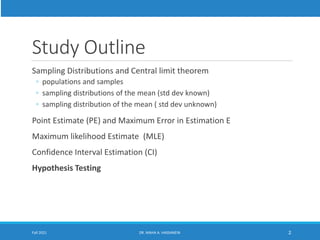
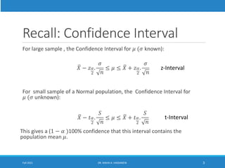
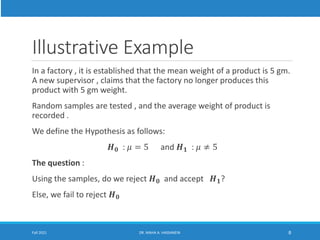
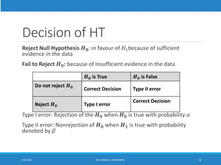
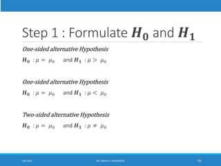
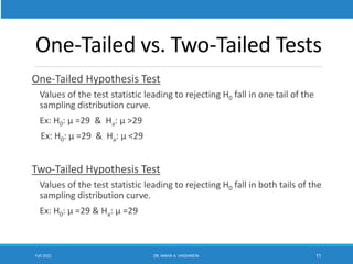
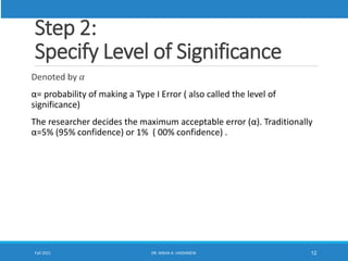
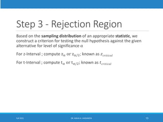
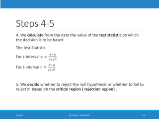
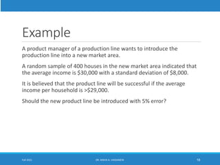
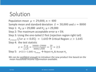
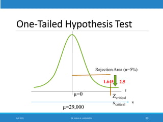
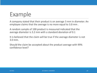
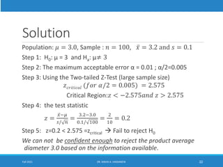
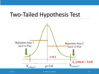
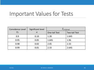
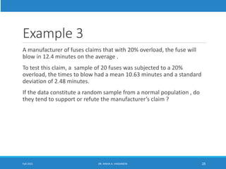
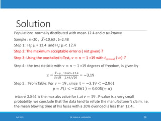
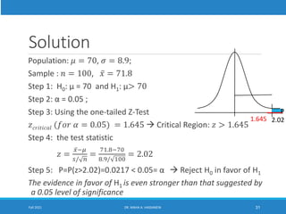
Lecture 15 - Hypothesis Testing (1).pdf

Study Outline
Sampling Distributions and Central limit theorem
◦ populations and samples
◦ sampling distributions of the mean (std dev known)
◦ sampling distribution of the mean ( std dev unknown)
Point Estimate (PE) and Maximum Error in Estimation E
Maximum likelihood Estimate (MLE)
Confidence Interval Estimation (CI)
Hypothesis Testing
Fall 2021 DR. MAHA A. HASSANEIN 2

Recall: Confidence Interval
For large sample , the Confidence Interval for 𝜇 (𝜎 known):
ത
𝑋 − 𝑧𝛼
2
.
𝜎
𝑛
≤ 𝜇 ≤ ത
𝑋 + 𝑧𝛼
2
.
𝜎
𝑛
For small sample of a Normal population, the Confidence Interval for
𝜇 (𝜎 unknown):
ത
𝑋 − 𝑡𝛼
2
.
𝑆
𝑛
≤ 𝜇 ≤ ത
𝑋 + 𝑡𝛼
2
.
𝑆
𝑛
This gives a (1 − 𝛼 )100% confidence that this interval contains the
population mean 𝜇.
z-Interval
t-Interval

Hypothesis Testing
We start by a conjecture or postulate something about a system
◦ For example ….
◦ Drinking coffee increases risk of cancer.
◦ There is a difference in accuracy between two measuring devices
◦ The sales of computer and the temperature are independent variables
◦ Blood type is independent on eye color.
Put the conjecture in the form of a statistical Hypothesis
We use the sample data to provide evidence that either accept or reject
the Hypothesis.
 Data-based Decision procedure

Hypothesis Testing
Definition
A statistical Hypothesis is an assertion or conjecture concerning one or
more populations.
In other words , a Hypothesis is a claim that we want to test

Illustrative Example
The proportion of defective parts in a lot is p=0.1 .
A random sample of size n =100 is tested for defective parts ; the
proportion of defective parts in the sample is found to be p=0.12
Does this Sample rejects the old believes that p=0.1 ? P>0.1 ? P<0.1
How certain are you?
If another random sample of size 100 , has p=0.2
Does this Sample rejects the old believes that p=0.1 ? How certain?

Types Of Hypothesis
Null Hypothesis , denoted by 𝐻0
Alternative Hypothesis , denoted by 𝐻1 ( or 𝐻𝑎)
Definitions.
𝐻1: Is question to be answered; the claim we wish to establish
“Research Question”
𝐻0: Is the logical complement of 𝐻1; we need to reject the claim
“Default” or “Current belief”

Illustrative Example
In a factory , it is established that the mean weight of a product is 5 gm.
A new supervisor , claims that the factory no longer produces this
product with 5 gm weight.
Random samples are tested , and the average weight of product is
recorded .
We define the Hypothesis as follows:
𝑯𝟎 : 𝜇 = 5 and 𝑯𝟏 : 𝜇 ≠ 5
The question :
Using the samples, do we reject 𝑯𝟎 and accept 𝑯𝟏?
Else, we fail to reject 𝑯𝟎

Decision of HT
Reject Null Hypothesis 𝑯𝟎: in favour of 𝐻1because of sufficient
evidence in the data
Fail to Reject 𝑯𝟎: because of insufficient evidence in the data
Type I error: Rejection of the 𝑯𝟎 when 𝑯𝟎 is true with probability 𝛼
Type II error: Nonrejection of 𝑯𝟎 when 𝑯𝟏 is true with probability
denoted by 𝛽
𝑯𝟎 is True 𝑯𝟎 is False
Do not reject 𝑯𝟎
Correct Decision Type II error
Reject 𝑯𝟎 Type I error
Correct Decision

Step 1 : Formulate 𝑯𝟎 and 𝑯𝟏
One-sided alternative Hypothesis
𝑯𝟎 : 𝜇 = 𝜇0 and 𝑯𝟏 : 𝜇 > 𝜇0
One-sided alternative Hypothesis
𝑯𝟎 : 𝜇 = 𝜇0 and 𝑯𝟏 : 𝜇 < 𝜇0
Two-sided alternative Hypothesis
𝑯𝟎 : 𝜇 = 𝜇0 and 𝑯𝟏 : 𝜇 ≠ 𝜇0

One-Tailed vs. Two-Tailed Tests
One-Tailed Hypothesis Test
Values of the test statistic leading to rejecting H0 fall in one tail of the
sampling distribution curve.
Ex: H0: µ =29 & Ha: µ >29
Ex: H0: µ =29 & Ha: µ <29
Two-Tailed Hypothesis Test
Values of the test statistic leading to rejecting H0 fall in both tails of the
sampling distribution curve.
Ex: H0: µ =29 & Ha: µ =29

Step 2:
Specify Level of Significance
Denoted by 𝛼
α= probability of making a Type I Error ( also called the level of
significance)
The researcher decides the maximum acceptable error (α). Traditionally
α=5% (95% confidence) or 1% ( 00% confidence) .

Step 3 - Rejection Region
Based on the sampling distribution of an appropriate statistic, we
construct a criterion for testing the null hypothesis against the given
alternative for level of significance α
For z-Interval ; compute zα or zα/2; known as 𝑧𝑐𝑟𝑖𝑡𝑖𝑐𝑎𝑙
For t-Interval ; compute tα or tα/2; known as 𝑡𝑐𝑟𝑖𝑡𝑖𝑐𝑎𝑙

Steps 4-5
4. We calculate from the data the value of the test statistic on which
the decision is to be based
The test Statistic
For z-Interval 𝑧 =
ҧ
𝑥−𝜇
𝜎/ 𝑛
For t-Interval 𝑡 =
ҧ
𝑥−𝜇
𝑠/ 𝑛
5. We decide whether to reject the null hypothesis or whether to fail to
reject it based on the critical region ( rejection region) .

Example
A product manager of a production line wants to introduce the
production line into a new market area.
A random sample of 400 houses in the new market area indicated that
the average income is $30,000 with a standard deviation of $8,000.
It is believed that the product line will be successful if the average
income per household is >$29,000.
Should the new product line be introduced with 5% error?

Solution
Population mean 𝜇 = 29,000, 𝑛 = 400
Sample mean and standard deviation ҧ
𝑥 = 30,000 and 𝑠 = 8000
Step 1: H0: µ = 29,000 and Ha: µ > 29,000
Step 2: The maximum acceptable error α = 5%
Step 3: Using the one-tailed Z-Test (rejection region right tail)
𝑧𝑐𝑟𝑖𝑡𝑖𝑐𝑎𝑙 (𝑓𝑜𝑟 𝛼 = 0.05) = 1.645 Critical Region: 𝑧 > 1.645
Step 4: the test statistic
𝑧 =
ҧ
𝑥−𝜇
𝑠/ 𝑛
=
30000−29000
8000/ 400
=
20
8
= 2.5
Step 5: z=2.5 > 1.645 =zcritical  Reject H0 & Accept Ha
We can be confident enough to introduce the new product line based on the
mean household income information available.

One-Tailed Hypothesis Test
µ=0
µ=29,000
Zcritical
xcritical
Rejection Area (α=5%)
1.645
z
x
2.5

Example
A company stated that their product is on average 3 mm in diameter. An
employee claims that the average is no more equal to 3.0 mm .
A random sample of 100 product is measured indicated that the
average diameter is 3.2 mm with a standard deviation of 0.1
It is believed that the claim will be true if the average diameter is not
3.0 mm.
Should the claim be accepted about the product average with 99%
confidence level?

Solution
Population: 𝜇 = 3.0, Sample : 𝑛 = 100, ҧ
𝑥 = 3.2 and 𝑠 = 0.1
Step 1: H0: µ = 3 and Ha: µ≠ 3
Step 2: The maximum acceptable error α = 0.01 ; α/2=0.005
Step 3: Using the Two-tailed Z-Test (large sample size)
𝑧𝑐𝑟𝑖𝑡𝑖𝑐𝑎𝑙 (𝑓𝑜𝑟 𝛼/2 = 0.005) = 2.575
Critical Region:𝑧 < −2.575𝑎𝑛𝑑 𝑧 > 2.575
𝑧 =
ҧ
𝑥−𝜇
𝑠/ 𝑛
=
3.2−3.0
0.1/ 100
=
2
10
= 0.2
Step 5: z=0.2 < 2.575 =zcritical  Fail to reject H0
We can not be confident enough to reject the product average
diameter 3.0 based on the information available.

Two-Tailed Hypothesis Test
µ=3.0
__
Xcritical 2
__
Xcritical 1
Rejection Area 1
(α/2=2.5%)
Rejection Area 2
(α/2=2.5%)
Z_critical = 2.645
z=0.2

Important Values for Tests
Convidence Level
CL
Significant level
𝛼
𝑍𝑐𝑟𝑖𝑡𝑖𝑐𝑎𝑙
One-tail Test Two-tail Test
0.9 0.10 1.28 1.645
0.95 0.05 1.645 1.96
0.98 0.02 2.05 2.33
0.99 0.01 2.33 2.645

Example 3
A manufacturer of fuses claims that with 20% overload, the fuse will
blow in 12.4 minutes on the average .
To test this claim, a sample of 20 fuses was subjected to a 20%
overload, the times to blow had a mean 10.63 minutes and a standard
deviation of 2.48 minutes.
If the data constitute a random sample from a normal population , do
they tend to support or refute the manufacturer’s claim ?

Solution
Population: normally distributed with mean 12.4 and 𝜎 𝑢𝑛𝑘𝑛𝑜𝑤𝑛
Sample : n=20 , ത
𝑋=10.63 , S=2.48
Step 1: H0: µ = 12.4 and Ha: µ < 12.4
Step 2: The maximum acceptable error α ( not given) ?
Step 3: Using the one-tailed t-Test, 𝜈 = 𝑛 − 1 =19 with 𝑡𝑐𝑟𝑖𝑡𝑖𝑐𝑎𝑙 𝛼 ?
Step 4: the test statistic with 𝜈 = 𝑛 − 1 =19 degrees of freedom, is given by
𝑡 =
ത
𝑋−𝜇
𝑆/ 𝑛
=
10.63−12.4
2.48/ 20
= −3.19
Step 5: From Table: For 𝜈 = 19 , since t = −3.19 < −2.861
𝑝 = 𝑃 𝑡 < −2.861 = 0.005(= 𝛼)
𝑤ℎ𝑒𝑟𝑒 2.861 is the max abs value for t at 𝜈 = 19 . P-value is a very small
probability, we conclude that the data tend to refute the manufacturer’s claim. i.e.
the mean blowing time of his fuses with a 20% overload is less than 12.4 .

𝑡𝛼
𝜈
𝛼

P-values in Hypothesis Testing
- Specify the rejection region whether we are two tail, one-tail
- Calculate your test statistic and compare
Purpose of the p-value is no different than before using rejection
regions
Before we have α and select the critical region accordingly .
The maximum risk of making type I error is controlled
Now P-values approach merely reject or donot reject conclusion with
probability p.
P-values approach are more common in research papers , real problems
, and applied statistics.

Definition: P-Value
A P-value is the lowest level (of significance) at which the observed value of
the test statistic is significant
i.e It is the probability of obtaining a sample “more extreme” than the ones
observed in your data, assuming that the Null Hypothesis is true .
Statistical Testing P-value Approach :
1- State Null and Alternative Hypothesis
2- Choose an appropriate test statistic
3- Compute P-value based on computed value of test statistic
Draw conclusions based on system
If p-value < α, we can reject H0 and accept Ha.
If p-value > α, we cannot reject H0 nor accept Ha.

Example 4
A random sample of 100 deaths in Us during the past year showed an
average life span of 71.8 years
A population with 𝜎 = 8.9 years , does this indicate that the mean life
span today is greater than 70 years? Use a 0.05 level of significance.

Solution
Population: 𝜇 = 70, 𝜎 = 8.9;
Sample : 𝑛 = 100, ҧ
𝑥 = 71.8
Step 1: H0: µ = 70 and H1: µ> 70
Step 2: α = 0.05 ;
Step 3: Using the one-tailed Z-Test
𝑧𝑐𝑟𝑖𝑡𝑖𝑐𝑎𝑙 (𝑓𝑜𝑟 𝛼 = 0.05) = 1.645  Critical Region: 𝑧 > 1.645
𝑧 =
ҧ
𝑥−𝜇
𝑠/ 𝑛
=
71.8−70
8.9/ 100
= 2.02
Step 5: P=P(z>2.02)=0.0217 < 0.05= α  Reject H0 in favor of H1
The evidence in favor of H1 is even stronger than that suggested by
a 0.05 level of significance
P
2.02
1.645

Reference
Text book
Chapter 7.
sec 7.4 Tests of Hypothesis
Sec. 7.5 Null Hypotheses and Tests of
Hypotheses
Sec. 7.6 Hypotheses concerning one mean
Sec. 7.7 The relation between Tests and
Confidence Intervals

Thank you for your attention
Maha

Lecture 15 - Hypothesis Testing (1).pdf

More Related Content

What's hot

Similar to Lecture 15 - Hypothesis Testing (1).pdf

Recently uploaded

Lecture 15 - Hypothesis Testing (1).pdf