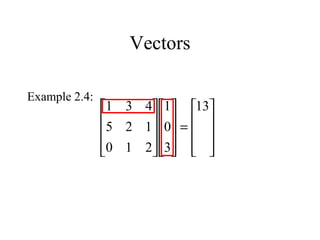
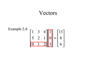
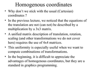
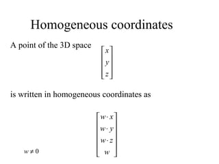
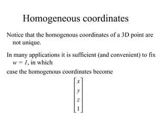
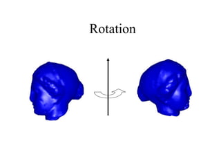
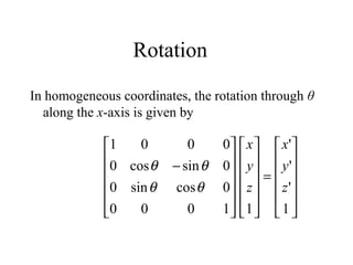
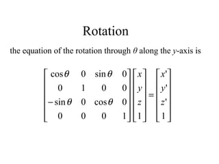
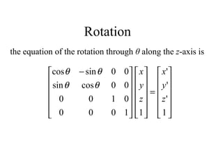
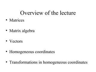
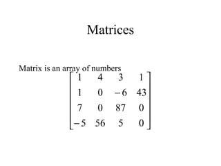
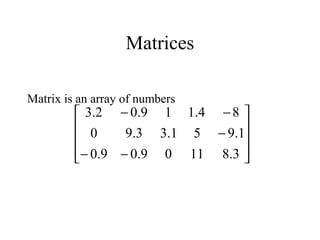
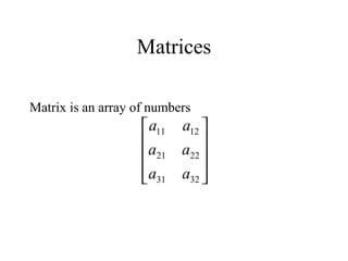
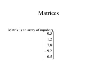
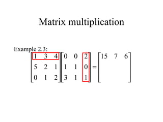
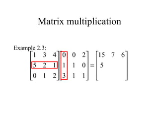
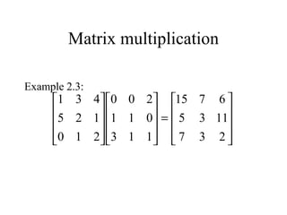
The document provides an overview of a lecture covering matrices, matrix algebra, vectors, homogeneous coordinates, and transformations in homogeneous coordinates. Key points include: matrices are arrays of numbers; operations on matrices include addition, multiplication by a scalar, and multiplication; vectors can represent points in space as column or row matrices; homogeneous coordinates allow points to be represented by 4D vectors, enabling translations and other transformations to be described by 4x4 matrices. This provides a unified approach for combining multiple transformations.


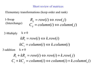

![Vectors
A column vector is a n x 1 matrix
A row vector is a 1 x n matrix
1
21
11
na
a
a
[ ]naaa 11211 ](https://image.slidesharecdn.com/matrices-170131045551/85/Matrices-27-320.jpg)
![Vectors
The point (x , y , z) of the 3D space can be written as
a column vector
or a row vector
z
y
x
[ ]zyx](https://image.slidesharecdn.com/matrices-170131045551/85/Matrices-28-320.jpg)