This document is a research project submitted to the University of Duhok examining matrices and their applications in solving systems of linear equations. The project begins with an introduction to basic matrix concepts such as types of matrices, operations on matrices, and finding the inverse and determinant of matrices. It then discusses how matrices can be used to solve different types of systems of linear equations, including homogeneous systems, Gaussian elimination, Gaussian-Jordan elimination, and Cramer's rule. The document contains acknowledgments, contents, abstract, and introduction sections before presenting the technical matrix concepts and methods for solving systems of linear equations.

1. UNIVERSITYOF DUHOK
FACLTY OF EDUATIONAL SCIENCE
SCHOOL OF BASEEDUCATION
DEPARTMWNT OF MATHMATICS
Matrices and its Applications to Solve Some
Methods of Systems of Linear Equations
A project submitted to thecouncilof Department of
Mathematics, School of Basic Education, Universityof Duhok, in
partial fulfillment of the requirement for B.Sc. degree of
mathematics
𝑷𝒓𝒆𝒑𝒂𝒓𝒆𝒅 𝒃𝒚: 𝑺𝒖𝒑𝒆𝒓𝒗𝒊𝒔𝒆𝒅 𝒃𝒚:
𝑨𝒃𝒅𝒂𝒍𝒍𝒂 𝑯𝒂𝒋𝒊 𝑴𝒖𝒘𝒂𝒇𝒂𝒒 𝑴𝒂𝒉𝒅𝒊 𝑺𝒂𝒍𝒊𝒉
𝑲𝒂𝒓𝒘𝒂𝒏 𝑯𝒂𝒕𝒎
1436 .A.H 2015.A.D 2715.K

2. Acknowledgement
First of all, thanks to Allah throughout all his almighty kindness,
and loveliness for letting us to finish our project.
We would like to express our thanks to our supervisor
𝑴𝒖𝒘𝒂𝒇𝒂𝒒 𝑴𝒂𝒉𝒅𝒊 𝑺𝒂𝒍𝒊𝒉 for giving us opportunity to write this research
under his friendly support. He made our research smoothly by his
discerning ideas and suggestions.
Also, we would like to thank all our friends and those people who
helped us during our work.

3. .
Contents
Chapter One
Basic Concepts in Matrix.
(1.1) Matrix…………………………………………………………….….....1
(1.2) Some Special Types of Matrices…………………..………....2
(1.3) Operations of Matrices…………………….……………..... ....11
(1.4) The Invers of a Square Matrix……………………………….17
(1.5) Some Properties of Determinants………………….…..….25
Chapter Two
System of Linear Equations
(2.1) Linear Equation………………………………………………………29
(2.2) Linear System……………………………………………………….....30
(2.2.1) Homogeneous System……………………………………….…..33
(2.2.2) Gaussian Elimination………………………………………….…34
(2.2.3) Gaussian-Jordan Elimination…………………………………35
(2.2.4) Cramer’s Rule………………………………………………….…...37
References…………………………………………………………….…………39

4. Abstract
In this research, we have tried to introduce matrix, its types and finding
inverse and determinant of matrix has involved. Then the applications of
matrices to some methods of solving systems of linear equations, such as
Homogeneous, Gaussian Elimination, Gaussian –jordan Elimination and
Cramer’s Rule, have been illustrated.

5. Introduction
Information in science and mathematics is often organized into rows
and columns to form rectangular arrays called "Matrices" (plural of
matrix). Matrices are often tables of numerical data that arise from
physical observation, but they also occur in various mathematical
contexts.
Linear algebra is a subject of crucial important to mathematicians and
users of mathematics. When mathematics is used to solve a problem it
often becomes necessary to find a solution to a so-called system of linear
equations. Applications of linear algebra are found in subjects as divers
as economic, physics, sociology, and management consultants use linear
algebra to express ideas solve problems, and model real activities.
The aim of writing this subject is to applying matrices to solve some
types of system of linear equations.
In the first chapter of this work matrices have introduced. Then
operations on matrices (such as addition and multiplication) where
defined and the concept of the matrix inverse was discussed. In the
second chapter theorems were given which provided additional insight
into the relationship between matrices and solution of linear systems.
Then we apply matrices to solve some methods of linear system such as
Homogeneous, Gaussian Elimination, Gaussian –jordan Elimination and
Cramer’s Rule.

6. CHAPTERONE
Basic Concepts in Matrix
In this chapter we begin our study on matrix, some special types of
matrix, operation of matrix, and finding invers and the determinant of
matrices.
(1.1) Matrix
An 𝑚 × 𝑛 matrix 𝐴 is rectangular array of 𝑚 × 𝑛 numbers arranged in 𝑚
rows and 𝑛 columns:
A=
[
a11 a12 ⋯ a1j ⋯ a1n
a21 a22 ⋯ a2j ⋯ a2n
⋮ ⋮ ⋮ ⋮
ai1 ai2 ⋯ aij ⋯ ain
⋮ ⋮ ⋮ ⋮
am1 am2 ⋯ amj ⋯ amn]
The 𝑖𝑗 𝑡ℎ
component of 𝐴 denoted 𝑎𝑖𝑗, is the number appearing in the
𝑖 𝑡ℎ
row and 𝑗 𝑡ℎ
column of 𝐴 we will some time write matrix 𝐴 as A=( 𝑎𝑖𝑗).
An m×n matrix is said to have the size m×n.
Examples:
(1) [
1 2
3 4
5 6
]
3×2
𝑚=3 , 𝑛=2 , (2) [
1 4 3 2 2
3 5 6 4 3
5 1 2 0 7
1 2 1 9 8
]
4×5
𝑚=4 , 𝑛=5

7. (1.2) SomeSpecialTypesof Matrices
1. SquareMatrix
The matrix which its number of rows equals to numbers of columns is
called square matrix. That is
A=[
𝑎11 𝑎12 ⋯ 𝑎1𝑛
𝑎21 𝑎22 ⋯ 𝑎2𝑛
⋮ ⋮ ⋮
𝑎 𝑚1 𝑎 𝑚2 ⋯ 𝑎 𝑚𝑛
]
m×n
When m=n then:
A= [
𝑎11 𝑎12 ⋯ 𝑎1𝑛
𝑎21 𝑎22 ⋯ 𝑎2𝑛
⋮ ⋮ ⋱ ⋮
𝑎 𝑛1 𝑎 𝑛2 ⋯ 𝑎 𝑛𝑛
] n×n
A is a square matrix
Example:
K=[
1 6 9
2 5 8
3 4 7
]
3×3
2. Unit (Identity) Matrix
The 𝑛 × 𝑛 matrix 𝐼 𝑛 =𝑎𝑖𝑗 , defined by 𝑎𝑖𝑗=1 if = 𝑗 , 𝑎𝑖𝑗=0 if 𝑖 ≠ 𝑗, is called
the 𝑛 × 𝑛 identity matrix .
𝐼=[
1 0 ⋯ 0
0 1 ⋯ 0
⋮ ⋮ ⋱ ⋮
0 0 ⋯ 1
]
Example: 𝐼2=[1 0
0 1
] , 𝐼3=[
1 0 0
0 1 0
0 0 1
]

8. Note: 𝐼𝐴 = 𝐴𝐼 = 𝐴
Example: 𝐴=[2 3
4 5
] , 𝐼=[1 0
0 1
]
𝐴𝐼=[2 3
4 5
] × [1 0
0 1
]=[
2 ∗ 1 + 3 ∗ 0 2 ∗ 0 + 3 ∗ 1
4 ∗ 1 + 5 ∗ 0 4 ∗ 0 + 5 ∗ 1
] = [2 3
4 5
]
𝐼𝐴=[1 0
0 1
] × [2 3
4 5
] = [1 ∗ 2 + 0 ∗ 4 1 ∗ 3 + 0 ∗ 5
0 ∗ 2 + 1 ∗ 4 0 ∗ 3 + 1 ∗ 5
] = [2 3
4 5
]
We note that 𝐼𝐴 = 𝐴𝐼 = 𝐴
3. Null(Zero) Matrix
A zero matrix is a matrix which its elements are zeros and is denoted by
the symbol 0 .
0 𝑚𝑛= [
0 0 … 0
0 ⋯ 0
⋮ ⋱ ⋮
0 ⋯ 0
]
Example:
Let 𝐴=[2 1 −3
4 5 8
] and 𝐵=[ 2 1
−3 4
]
We see that
𝐴 +023=[2 1 −3
4 5 8
]+[0 0 0
0 0 0
]=[2 1 −3
4 5 8
]=𝑨
𝐵022=[ 2 1
−3 3
] [0 0
0 0
]=[0 0
0 0
]=022
Property of ZeroMatrix
 𝐴 + 0 = 0 + 𝐴 = 𝐴
 𝐴 − 𝐴 = 0
 0 − 𝐴 = −𝐴
 0𝐴 = 0 , 𝐴0 = 0

9. 4. DiagonalMatrix
Diagonal matrix is a square matrix in which all the elements not on the
main diagonal are zeros.
A=[
𝑎11 0 ⋯ 0
0 𝑎22 ⋯ 0
⋮ ⋮ ⋱ ⋮
0 0 ⋯ 𝑎33
]
The elements of a square matrix 𝐴 where the subscripts are equal,
namely 𝑎11, 𝑎22, … , 𝑎 𝑛𝑛, form the main diagonal.
Example:
A=[
1 0 0
0 2 0
0 0 3
] , main diagonal=1,2,3
5. CommutativeMatrix
We say that the matrices 𝐴 and 𝐵 are commutative under the operation
product if 𝐴 and 𝐵 are square matrices and
𝐴. 𝐵 = 𝐵. 𝐴 and we say that 𝐴 𝑎𝑛𝑑 𝐵 are invertible commutative if 𝐴
and 𝐵 are square matrices and 𝐴. 𝐵 = 𝐵. 𝐴 .
Example:
𝐴 = [5 1
1 5
] , 𝐵 = [2 4
4 2
]
𝐴. 𝐵 = [5 1
1 5
] [2 4
4 2
] = [
10 + 4 20 + 2
2 + 20 4 + 10
] = [14 22
22 14
]
𝐵. 𝐴 = [2 4
4 2
] [5 1
1 5
] = [
10 + 4 2 + 20
20 + 2 4 + 10
] = [14 22
22 14
]
Then 𝐴. 𝐵 = 𝐵. 𝐴

10. Note: A square matrix 𝐴 is said to be invertibleif there exists 𝐵 such that
𝐴𝐵 = 𝐵𝐴 = 𝐼. 𝐵 is denoted 𝐴−1
and is unique.
If 𝑑𝑒𝑡(𝐴) = 0 then a matrix is not invertible.
6. TriangularMatrix
A square matrix 𝐴 is 𝑛 × 𝑛 , (𝑛 ≥ 3), is triangular matrix iff 𝑎𝑖𝑗 =0
when 𝑖 ≥ 𝑗 + 1 ,or 𝑗 ≥ 𝑖 + 1.
The are two type of triangular matrices:
i. Upper Triangular Matrix
A square matrix is called an upper triangular matrix if all the elements
below the main diagonal are zero.
Example:
𝐴=[
1 5 9
0 2 1
0 0 3
]
ii. Lower Triangular Matrix
A square matrix is called lower triangular matrix if all the elements above
the main diagonal are zero.
Example:
𝐴=[
1 0 0
6 2 0
9 7 3
]
Transpose of Matrix
Transpose of 𝑚 × 𝑛 matrix 𝐴 ,denoted 𝐴 𝑇
or 𝐴̀, is 𝑛 × 𝑚 matrix with
( 𝐴𝑖𝑗)
𝑇
= 𝐴𝑗𝑖

11. 𝐴=[
𝑎11 𝑎12 ⋯ 𝑎1𝑛
𝑎21 𝑎22 ⋯ 𝑎2𝑛
⋮ ⋮ ⋮
𝑎 𝑚1 𝑎 𝑚2 ⋯ 𝑎 𝑚𝑛
]
m×n
, 𝐴 𝑇
=[
𝑎11 𝑎21 ⋯ 𝑎 𝑚1
𝑎12 𝑎22 ⋯ 𝑎 𝑚2
⋮ ⋮ ⋮
𝑎1𝑛 𝑎2𝑛 ⋯ 𝑎 𝑚𝑛
]
n×m
row and columns of 𝐴 are transposed in 𝐴 𝑇
Example:
𝐴 = [
0 4
7 0
3 1
] , 𝐴 𝑇
= [0 7 3
4 0 1
]
Note: transpose converts row vectors to column vector , vice versa.
 Properties of Transpose
Let 𝐴 and 𝐵 be matrix and 𝑐 be a scalar. Assume that the size of the
matrix are such that the operations can be performed.
 ( 𝐴 + 𝐵) 𝑇
= 𝐴 𝑇
+ 𝐵 𝑇
Transpose of the sum
 ( 𝑐𝐴) 𝑇
= 𝑐𝐴 𝑇
Transpose of scalar multiple
 ( 𝐴𝐵) 𝑇
= 𝐵 𝑇
𝐴 𝑇
Transpose of a product
 ( 𝐴 𝑇) 𝑇
= 𝐴
7. SymmetricMatrix
A real matrix 𝐴 is called symmetric if 𝐴 𝑇
= 𝐴. In other words 𝐴 is square
(𝑛 × 𝑛 )and 𝑎𝑖𝑗 = 𝑎𝑗𝑖 for all 1 ≤ 𝑖 ≤ 𝑛, 1 ≤ 𝑗 ≤ 𝑛.
Example:
𝐴=[
1 0 5
0 2 6
5 6 3
] 𝐴 𝑇
=[
1 0 5
0 2 6
5 6 3
]
Note: if 𝐴 = 𝐴 𝑇
then 𝐴 is a symmetric matrix
8. Skew-Symmetric Matrix

12. Areal matrix 𝐴 is called Skew-Symmetricif 𝐴 𝑇
= −𝐴 . In other words 𝐴 is
square (𝑛 × 𝑛) and 𝑎𝑗𝑖=−𝑎𝑖𝑗 for all 1 ≤ 𝑖 ≤ 𝑛, 1 ≤ 𝑗 ≤ 𝑛
Example:
A=[
0 5 6
−5 0 8
−6 −6 0
] − 𝐴=[
0 −5 −6
5 0 −8
6 8 0
]
A=[
0 5 6
−5 0 8
−6 −8 0
] 𝐴 𝑇
=[
0 −5 −6
5 0 −8
6 8 0
] ∴ 𝐴 𝑇
= −𝐴
Determinants of Matrix
The determinant of a square matrix 𝐴 = [𝑎𝑖𝑗] is a number denoted by |A|
or 𝑑𝑒𝑡(𝐴) , through which important properties such as singularity can
be briefly characterized .
This number is defined as the following function of the matrix elements:
|𝐴| = 𝑑𝑒𝑡(𝐴) = ± ∏ 𝑎1𝑗1
𝑎2𝑗2
… 𝑎 𝑛𝑗 𝑛
Where the column indices 𝑗1, 𝑗2, …, 𝑗 𝑛 are taken from the set {1,2,…,n}
with no repetitions allowed . The plus (minus) sign is taken if the
permutation (𝑗1 𝑗2 … 𝑗 𝑛) is even (odd).
Someproperties of determinants willbe discussed later inthis
chapter
9. Singular and Nonsingular Matrix
A square matrix 𝐴 is said to be singular if 𝑑𝑒𝑡(𝐴) = 0 .
𝐴 is nonsingular if 𝑑𝑒𝑡(𝐴) ≠ 0.
Theorem:
Let 𝐴 be a square matrix. Then 𝐴 is a singular if
(a) all elements of a row (column) are zero.
(b) two rows (column) are equal.
(c) two rows(column) are proportional.

13. Note: (b) is a special case of (c) , but we list it separately to give it special
emphasis.
Example: we show that the following matrices are singular.
(a) A=[
2 0 −7
3 0 1
−4 0 9
] (b) B=[
2 −1 3
1 2 4
2 4 8
]
(a) All the elements in column 2 of A are zero. Thus 𝑑𝑒𝑡 = 0.
(b) Observe that every element in row 3 of B is twice the
corresponding element in row 2. We write
(row 3) = 2(row 2)
Row 2 and 3 are proportional. Thus 𝑑𝑒𝑡(𝑏) = 0.
10. OrthogonalMatrix
we say that a matrix 𝐴 is orthogonal if 𝐴. 𝐴 𝑇
= 𝐼 = 𝐴 𝑇
. 𝐴
Example:
𝐴 =
[
1 0 0
0
1
2
√3
2
0 −
√3
2
1
2 ]
, 𝐴 𝑇
=
[
1 0 0
0
1
2
−
√3
2
0
√3
2
1
2 ]
𝐴. 𝐴 𝑇
=
[
1 0 0
0
1
2
√3
2
0 −
√3
2
1
2 ]
.
[
1 0 0
0
1
2
−
√3
2
0
√3
2
1
2 ]
=
[
1 0 0
0
1
4
+
3
4
1
2
.
−√3
2
+
√3
2
.
1
2
0
−√3
2
.
1
2
+
1
2
.
√3
2
3
4
.
1
4 ]
= [
1 0 0
0 1 0
0 0 1
] = 𝐼
∴ 𝐴 is orthogonal matrix

14. 11. 𝐓𝐨𝐞𝐩𝐥𝐢𝐭𝐳Matrix
A matrix 𝐴 is said to be 𝐓𝐨𝐞𝐩𝐥𝐢𝐬𝐥𝐢𝐭𝐳 if it has common elements on their
diagonals, that is 𝑎𝑖,𝑗=𝑎𝑖+1 ,𝑗+1
Example: A=[
5 6 2
0 5 6
3 0 5
]
Where 𝑎11=𝑎22=𝑎33=5
𝑎12=𝑎23=6
𝑎21=𝑎32=0
12. Nilpotent Matrix
A square matrix 𝐴 is said to nilpotent if there is a positive integer 𝑝 such
that 𝐴 𝑃
= 0. The integer 𝑝 is called the degree of 𝑛𝑖𝑙𝑝𝑜𝑡𝑒𝑛𝑐𝑦 of the
matrix.
Example:
𝐴 = [
1 −3 −4
−1 3 4
1 −3 −4
] , 𝑝 = 2
𝐴2
= 0
𝐴. 𝐴 = [
1 −3 −4
−1 3 4
1 −3 −4
] . [
1 −3 −4
−1 3 4
1 −3 −4
] = [
0 0 0
0 0 0
0 0 0
]
13. Periodic (Idempotent) Matrix
A matrix 𝐴 is said to be periodic , that period (order) 𝐾 , if 𝐴 is satisfy
𝐴 𝐾+1
= 𝐴 and if 𝐾 = 1 then 𝐴2
= 𝐴 so 𝐴 is called idempotent matrix.
Example:

15. 𝐴 = [
1 −2 −6
−3 2 9
2 0 −3
] , 𝐾 = 2
𝐴 𝐾+1
= 𝐴2+1
= 𝐴3
𝐴. 𝐴 = [
−5 −6 −6
9 10 9
−4 −4 −3
] , 𝐴2
. 𝐴 = [
1 −2 −6
−3 2 9
2 0 3
]
∴ 𝐴 is idempotent matrix
14. StochasticMatrix
An 𝑛 × 𝑛 matrix 𝐴 is called stochastic if each element is a number
between 0 and 1 and each column of 𝐴 adds up to 1.
A=
[
1
4
1
3
0
1
2
2
3
3
4
1
4
0
1
4]
,
∑ column(1) =1 , ∑column( 2) = 1 , ∑ column( 3) = 1
15. TraceMatrix
Let 𝐴 be a square matrix, the trace of 𝐴 denoted 𝑡𝑟(𝐴) is the sum of the
diagonal elements of 𝐴 .Thus if 𝐴 is an 𝑛 × 𝑛 matrix.
𝒕𝒓(𝑨) = 𝒂 𝟏𝟏 + 𝒂 𝟐𝟐 + ⋯ + 𝒂 𝒏𝒏
Example:

16. The trace of the matrix 𝐴 =[
4 1 −2
2 −5 6
7 3 0
].
is, 𝑡𝑟(𝐴) = 4 + (−5) + 0 = −1
Properties of Trace
Let 𝐴 and 𝐵 be matrix and 𝑐 be a scalar, assume that the sizes of the
matrices are such that the operations can be performed.
 𝑡𝑟( 𝐴 + 𝐵) = 𝑡𝑟(𝐴) + 𝑡𝑟(𝐵)
 𝑡𝑟(𝐴𝐵) = 𝑡𝑟(𝐵𝐴)
 𝑡𝑟(𝑐𝐴) = 𝑐𝑡𝑟(𝐴)
 𝑡𝑟( 𝐴) 𝑇
= 𝑡𝑟(𝐴)
Note: if A is not square that the trace is not defined.
16. 𝑯𝒆𝒓𝒎𝒊𝒕𝒊𝒂𝒏 Matrix
A square matrix A is said to be 𝒉𝒆𝒓𝒎𝒊𝒕𝒊𝒂𝒏 if A̅T=A.
Note: The conjugate of a complex number 𝑧 = 𝑎 + 𝑖𝑏 is defined and
written z̅=a-ib .
Example:
A=[
3 7 + 𝑗2
7 − 𝑗2 −2
] ,is ℎ𝑒𝑟𝑚𝑖𝑡𝑖𝑎𝑛
Taking the complex conjugates of each of the elements in 𝐴 gives
A̅=[
3 7 − 𝑗2
7 + 𝑗2 −2
]
Now taking the transposes of A , we get
A̅T=[
3 7 + 𝑗2
7 − 𝑗2 −2
]
So we can see that A̅T=A

17. (1.3) Operations ofMatrices
1. Addition
If 𝐴 and 𝐵 are m × n matrices such that
𝐴=[
𝑎11 𝑎12 ⋯ 𝑎1𝑛
𝑎21 𝑎22 ⋯ 𝑎2𝑛
⋮ ⋮ ⋮
𝑎 𝑚1 𝑎 𝑚2 ⋯ 𝑎 𝑚𝑛
]
m×n
and 𝐵= [
𝑏11 𝑏12 ⋯ 𝑏1𝑛
𝑏21 𝑏22 ⋯ 𝑏2𝑛
⋮ ⋮ ⋮
𝑏 𝑚1 𝑏 𝑚2 ⋯ 𝑏 𝑚𝑛
]
m×n
Then 𝐴 + 𝐵=[
𝑎11 + 𝑏11 𝑎12 + 𝑏12 ⋯ 𝑎1𝑛 + 𝑏1𝑛
𝑎21 + 𝑏21 𝑎22 + 𝑏22 ⋯ 𝑎2𝑛 + 𝑏2𝑛
⋮ ⋮ ⋱ ⋮
𝑎 𝑚1 + 𝑏 𝑚1 𝑎 𝑚2 + 𝑏 𝑚2 ⋯ 𝑎 𝑚𝑛 + 𝑏 𝑚𝑛
]
Note: Addition of matrices of different sizes is not defined.
Example: [
0 4
7 0
3 1
]+[
1 2
2 3
0 4
]=[
1 6
9 3
3 5
]
Properties of Matrix Addition
 𝐴 + 𝐵 = 𝐵 + 𝐴 (commutative)
 (𝐴 + 𝐵) + 𝐶 = 𝐴 + (𝐵 + 𝐶) (associative), so we can write as
𝐴 + 𝐵 + 𝐶
 𝐴 + 0 = 0 + 𝐴 = 𝐴
 ( 𝐴 + 𝐵) 𝑇
= 𝐴 𝑇
+ 𝐵 𝑇
2. Subtraction
Matrix subtraction is defined for two matrix 𝐴 = [𝑎𝑖𝑗] and 𝐵 = [𝑏𝑖𝑗] of the
same size in the usual way; that is
𝐴 − 𝐵 = [𝑎𝑖𝑗] − [ 𝑏𝑖𝑗 ] = [ 𝑎𝑖𝑗 − 𝑏𝑖𝑗].
If 𝐴 and 𝐵 m × n matrix such that

18. 𝐴=[
𝑎11 𝑎12 ⋯ 𝑎1𝑛
𝑎21 𝑎22 ⋯ 𝑎2𝑛
⋮ ⋮ ⋮
𝑎 𝑚1 𝑎 𝑚2 ⋯ 𝑎 𝑚𝑛
]
m×n
and 𝐵= [
𝑏11 𝑏12 ⋯ 𝑏1𝑛
𝑏21 𝑏22 ⋯ 𝑏2𝑛
⋮ ⋮ ⋮
𝑏 𝑚1 𝑏 𝑚2 ⋯ 𝑏 𝑚𝑛
]
m×n
Then 𝐴 − 𝐵=[
𝑎11 − 𝑏11 𝑎12 − 𝑏12 ⋯ 𝑎1𝑛 − 𝑏1𝑛
𝑎21 − 𝑏21 𝑎22 − 𝑏22 ⋯ 𝑎2𝑛 − 𝑏2𝑛
⋮ ⋮ ⋱ ⋮
𝑎 𝑚1 − 𝑏 𝑚1 𝑎 𝑚2 − 𝑏 𝑚2 ⋯ 𝑎 𝑚𝑛 − 𝑏 𝑚𝑛
]
Note: Subtraction of matrices of different sizes is not defined.
Example:
[
0 4
7 0
3 1
]-[
1 2
2 3
0 4
]=[
−1 2
5 −3
3 −3
]
3. Negative
Consider 𝐶 to be a matrix, the negative of 𝐶 denoted by −𝐶 , which
defined as (−1)𝐶, Where each element in 𝐶 is multiplied by (−1).
Example:
𝐶 = [3 −2 4
7 −3 0
]. Then – 𝐶 = [−3 2 −4
−7 3 0
].
4. Multiplication
We can product two matrices 𝐴 and 𝐵 if the number of column in a
matrix 𝐴 be equal to the number of rows in a matrix 𝐵.The element in
row 𝑖 and column 𝑗 of 𝐴𝐵 is obtained by multiplying the corresponding
element of row 𝑖 of 𝐴 and column 𝑗 of 𝐵 and adding the products.
[
.
.
.
] 𝐵 is 3 × 𝑛
𝐴 is 𝑚 × 3 [
. . .
] [
. ] 𝐴𝐵 is 𝑚 × 𝑛

19. Note: The product of 𝐴 and 𝐵 con not be obtained if the number of
columns in 𝐴 does not equal the number of rows in 𝐵.
Let 𝐴 have 𝑛 columns and 𝐵 have 𝑛 rows .The 𝑖 𝑡ℎ
row of 𝐴 is
[𝑎𝑖1 𝑎𝑖2 …𝑎𝑖𝑛] and the 𝑗 𝑡ℎ
column of 𝐵 is
[
𝑏1𝑗
𝑏2𝑗
⋮
𝑏 𝑛𝑗]
.
Thus if = 𝐴𝐵 , then 𝑐𝑖𝑗=𝑎𝑖1 𝑏1𝑗 +𝑎𝑖2 𝑏2𝑗+…+𝑎𝑖𝑛 𝑏 𝑛𝑗 .
Propertiesof MatrixMultiplication
 0𝐴 = 0, 𝐴0 = 0 (here 0 can be scalar, or a compatible matrix)
 𝐼𝐴 = 𝐴𝐼 = 𝐴
 (𝐴𝐵)𝐶 = 𝐴(𝐵𝐶), so we can write as 𝐴𝐵𝐶
 α(AB)=( αA)B , where 𝛼 is a scalar
 𝐴(𝐵 + 𝐶) = 𝐴𝐵 + 𝐴𝐶 ,(𝐴 + 𝐵)𝐶 = 𝐴𝐶 + 𝐵𝐶
 ( 𝐴𝐵) 𝑇
= 𝐵 𝑇
𝐴 𝑇
ScalarMultiplication
let 𝐴 be a matrix and 𝑐 be a scalar, the scalar multiple of 𝐴 by 𝑐, denoted
𝑐𝐴 , is the matrix obtained by multiplying every element of 𝐴 by 𝑐, the
matrix 𝑐𝐴 will be the same size of 𝐴.
Thus if 𝐵 = 𝐶𝐴 , then 𝑏𝑖𝑗 =c𝑎𝑖𝑗.
Example: let 𝐴=[1 −2 4
7 −3 0
],determine 3𝐴.
Then
Now multiple every element of 𝐴 by 3 we get

20. 3𝐴 = [ 3 −6 12
21 −9 0
].
Observe that 𝐴 and 3𝐴 are both 2 × 3 matrix
Remark:
If 𝐴 is a square matrix, then 𝐴 multiplied by itself 𝑘 times is written Ak.
𝐴 𝑘
= 𝐴𝐴 … 𝐴 , 𝐾 times
Familiar rules of exponents of real numbers hold for matrices.
Theorem:
If 𝐴 is an 𝑛 × 𝑛 square matrix and 𝑟 and 𝑠 are nonnegative integers, then
1. 𝐴 𝑟
𝐴 𝑠
= 𝐴 𝑟+𝑠
2. ( 𝐴 𝑟) 𝑠
= 𝐴 𝑟𝑠
3. 𝐴0
= 𝐼 𝑛 (by definition)
We verify the first rule, the proof of the second rule is similar
𝐴 𝑟
𝐴 𝑠
= 𝐴 … 𝐴⏟
𝑟 𝑡𝑖𝑚𝑒𝑠
𝐴 … 𝐴⏟
𝑠 𝑡𝑖𝑚𝑒𝑠
= 𝐴 … 𝐴⏟
𝑠+𝑟 𝑡𝑖𝑚𝑒𝑠
= 𝐴 𝑟+𝑠
Example: If = [ 1 −2
−1 0
] , compute 𝐴4
.
This example illustrates how the above rules can be used to reduce the
amount of computation involved in multiplying matrices. We know that
𝐴4
= 𝐴𝐴𝐴𝐴. We could perform three matrix multiplication to arrive at 𝐴4
.
However we con apply rule 2 above to write 𝐴4
= ( 𝐴2)2
and thus arrive
at the result using two products. We get
𝐴2
= [ 1 −2
−1 0
] [ 1 −2
−1 0
] = [ 3 −2
−1 2
]
𝐴4
= [ 3 −2
−1 2
] [ 3 −2
−1 2
] = [11 −10
−5 6
]
The usual index laws hold provided 𝐴𝐵 = 𝐵𝐴

21.  ( 𝐴𝐵) 𝑛
= 𝐴 𝑛
𝐵 𝑛
 𝐴 𝑚
𝐵 𝑛
= 𝐵 𝑛
𝐴 𝑚
 ( 𝐴 + 𝐵)2
= 𝐴2
+ 2𝐴𝐵 + 𝐵2
 ( 𝐴 + 𝐵) 𝑛
= ∑ ( 𝑛
𝑖
)𝑛
𝑖=0 𝐴𝑖
𝐵 𝑛−𝑖
 (𝐴 + 𝐵)(𝐴 − 𝐵) = 𝐴2
– 𝐵2
We now state basic of the natural numbers.
Equality
The matrix 𝐴 and 𝐵 are said to be equal if 𝐴 and 𝐵 have the same size and
corresponding element are equal; that is 𝐴 and 𝐵 ∈ 𝑀(𝑚 × 𝑛) and 𝐴 =
[𝑎𝑖𝑗] , 𝐵 = [𝑏𝑖𝑗 ] with 𝑎𝑖𝑗 =𝑏𝑖𝑗 for 1 ≤ 𝑖 ≤ 𝑚 , 1 ≤ 𝑗 ≤ 𝑛.
Example:
𝐴 = [
1 2 3
4 5 6
7 8 9
] , 𝐵 = [
3 1 2
4 5 6
7 8 9
] , 𝐶 = [
1 1 + 1 3
4 5
12
2
7 5 + 3 3 ∗ 3
]
𝐴 = 𝐶
Minor
Let 𝐴 be an 𝑛 × 𝑛 square matrix obtained from 𝐴 by deleting the 𝑖 𝑡ℎ
row
and 𝑗 𝑡ℎ
column of 𝐴 𝑀𝑖𝑗is called the 𝑖𝑗 𝑡ℎ
minor of 𝐴 .
𝐴 = [
𝑎11 𝑎12 𝑎13
𝑎21 𝑎22 𝑎23
𝑎31 𝑎32 𝑎33
]
𝑀11 = [
𝑎22 𝑎23
𝑎32 𝑎33
] , 𝑀12 = [
𝑎21 𝑎23
𝑎31 𝑎33
] , 𝑀13 = [
𝑎21 𝑎22
𝑎31 𝑎32
]
Cofactors

22. The cofactor 𝑐𝑖𝑗 is defined as the coefficient of 𝑎𝑖𝑗 in the determinant 𝐴
If is given by the formula
𝐶𝑖𝑗=(−1)𝑖+𝑗
𝑚𝑖𝑗
Where the minor is the determinant of order (𝑛 − 1) × (𝑛 − 1) formed
by deleting the column and row containing 𝑎𝑖𝑗.
𝑐11=(−1)1+1
𝑚11=+1. [
𝑎11 𝑎12 𝑎13
𝑎21 𝑎22 𝑎23
𝑎31 𝑎32 𝑎33
] =+1. |
𝑎22 𝑎23
𝑎32 𝑎33
| = 𝑎22 𝑎33-𝑎32 𝑎23
𝑐12=(−1)1+2
𝑚12= -1. [
𝑎11 𝑎12 𝑎13
𝑎21 𝑎22 𝑎23
𝑎31 𝑎32 𝑎33
]=-1. |
𝑎21 𝑎23
𝑎31 𝑎33
| = 𝑎21 𝑎33-𝑎31 𝑎23
𝑐13=(−1)1+3
𝑚13=+1. [
𝑎11 𝑎12 𝑎13
𝑎21 𝑎22 𝑎23
𝑎31 𝑎32 𝑎33
]=+1. |
𝑎21 𝑎22
𝑎31 𝑎32
| = 𝑎21 𝑎32-𝑎31 𝑎22
Definition:
Let 𝐴 be 𝑛 × 𝑛 matrix and 𝑐𝑖𝑗 be the cofactor of 𝑎𝑖𝑗.The matrix whose
(𝑖, 𝑗) 𝑡ℎ
element is 𝑐𝑖𝑗 is called the matrix of the cofactors of 𝐴. The
transpose of this matrix is called the 𝒂𝒅𝒋𝒐𝒊𝒏𝒕 of A and is denoted 𝒂𝒅𝒋(𝑨).
[
c11 c12 ⋯ c1n
c21 c22 ⋯ c2n
⋮ ⋮ ⋱ ⋮
cn1 cn2 ⋯ cnn
] [
c11 c12 ⋯ c1n
c21 c22 ⋯ c2n
⋮ ⋮ ⋱ ⋮
cn1 cn2 ⋯ cnn
]
𝑇
𝑀𝑎𝑡𝑟𝑖𝑥 𝑜𝑓 𝑐𝑜𝑓𝑎𝑐𝑡𝑜𝑟𝑠 𝐴𝑑𝑗𝑜𝑖𝑛𝑡 𝑚𝑎𝑡𝑟𝑖𝑥
Example: give the matrix of the cofactors and the 𝑎𝑑𝑗𝑜𝑖𝑛𝑡 matrix of the
following matrix A.
A=[
2 0 3
−1 4 −2
1 −3 5
]
The cofactor of A are as follows.
𝑐11=| 4 −2
−3 5
|=14 , 𝑐12=− |−1 −2
1 5
|=3 , 𝑐13=|−1 4
1 −3
|=-1
𝑐21=− | 0 3
−3 5
|=-9 , 𝑐22=|2 3
1 5
|=7 , 𝑐23=− |2 0
1 −3
|=6

23. 𝑐31=|0 3
4 −2
|=-12 , 𝑐32=− | 2 3
−1 −2
|=1 , 𝑐33=| 2 0
−1 4
|=8
The matrix of cofactors of 𝐴 is [
14 3 −1
−9 7 6
−12 1 8
]
The 𝑎𝑑𝑗𝑜𝑖𝑛𝑡 of 𝐴 is the transpose of this matrix
𝑎𝑑𝑗(𝐴)= [
14 −9 −12
3 7 1
−1 6 8
]
(1.4)TheInverseof a SquareMatrix
The inverse 𝑎−1
of a scalar (= 𝑎 number) 𝑎 is defined by
𝑎 𝑎−1
= 1.
For square matrices we use a similar definition the inverse
𝐴−1
of a 𝑛 × 𝑛 matrix 𝐴 fulfils the relation
𝐴𝐴−1
= 𝐼
where 𝐼 is the 𝑛 × 𝑛 unit matrix defined earlier.
Example: we show that, as usual, the identity matrix of the appropriate
size. 𝐴 = [−1 1
−2 0
] , 𝐵 =
1
2
[0 −1
2 −1
]
All we need do is to check that 𝐴𝐵 = 𝐵𝐴 = 𝐼
𝐴𝐵 = [−1 1
−2 0
] ×
1
2
[0 −1
2 −1
] =
1
2
[0 −1
2 −1
] × [−1 1
−2 0
] =
1
2
[2 0
0 2
]
= [1 0
0 1
]
The reader should check that 𝐴𝐵 = 𝐼 also
Note: if 𝐴−1
exists then
𝑑𝑒𝑡(𝐴)𝑑𝑒𝑡(𝐴−1
) = 𝑑𝑒𝑡(𝐴𝐴−1
) = 𝑑𝑒𝑡(𝐼) = 1

24. Hence 𝑑𝑒𝑡(𝐴−1
) = ( 𝑑𝑒𝑡𝐴)−1
Example: 𝐴 = [3 7
2 6
]
𝑑𝑒𝑡(𝐴) = 18 − 14 = 4 ,( 𝑑𝑒𝑡( 𝐴))
−1
=
1
4
𝐴−1
=
1
4
[ 6 −7
−2 3
] = [
6
4
−7
4
−2
4
3
4
]
𝑑𝑒𝑡(𝐴−1
) =
18
16
−
14
16
=
4
16
=
1
4
∴ 𝑑𝑒𝑡(𝐴−1
) = ( 𝑑𝑒𝑡𝐴)−1
,
1
4
=
1
4
Remark:
 Non-square matrices do not have an inverse.
 The inverse of A is usually written 𝐴−1
.
 Not all square matrices have an inverse.
 A square matrix 𝐴 is invertible if and only if 𝑑𝑒𝑡(𝐴) ≠ 0.
 𝐴−1
exists if and only if 𝐴 is nonsingular.
FindingInverseofMatrix
1- The Inverse of a 𝟐 × 𝟐 Matrix
If 𝑎𝑑 − 𝑏𝑐 ≠ 0 then the 2 × 2 matrix 𝐴 = [ 𝑎 𝑏
𝑐 𝑑
] has a (unique)
inverse given by
𝐴−1
=
1
𝑎𝑑−𝑏𝑐
[ 𝑑 −𝑏
−𝑐 𝑎
]
Note: 𝑎𝑑 − 𝑏𝑐 = 0 that 𝐴 has no inverse.

25. In words: to find the inverse of a 2 × 2 matrix 𝐴 we effectively
interchange the diagonal elements 𝑎 and 𝑑, change the sign of the other
two elements and then divide by the determinant of 𝐴.
Example: 𝐴 = [3 7
2 6
]
𝑑𝑒𝑡(𝐴) = 18 − 14 = 4 , 𝐴−1
=
1
4
[ 6 −7
−2 3
] = [
6
4
−7
4
−2
4
3
4
]
2- The Inverseof a 3×3 Matrix-TheDeterminant Method
Given a square matrix 𝐴:
 Find 𝑑𝑒𝑡(𝐴), if det(𝐴)=0 then ,as we know 𝐴−1
does not exists. If
det(𝐴)≠0 we can proceed to find the inverse matrix.
 Replace each element of 𝐴 by its cofactor
𝐶11=[
𝑎22 𝑎23
𝑎32 𝑎33
], 𝐶12=[
𝑎21 𝑎23
𝑎31 𝑎33
] , 𝐶13=[
𝑎21 𝑎22
𝑎31 𝑎32
]
𝐶21=[
𝑎12 𝑎13
𝑎32 𝑎33
] , 𝐶22=[
𝑎11 𝑎13
𝑎31 𝑎33
], 𝐶23=[
𝑎11 𝑎12
𝑎31 𝑎32
]
𝐶31=[
𝑎12 𝑎13
𝑎22 𝑎23
], 𝐶32=[
𝑎11 𝑎13
𝑎21 𝑎23
], 𝐶33=[
𝑎11 𝑎12
𝑎21 𝑎22
]
Cofactor =[
𝐶11 𝐶12 𝐶13
𝐶21 𝐶22 𝐶23
𝐶31 𝐶32 𝐶33
] =𝐴
 Transpose the result to form the 𝒂𝒅𝒋𝒐𝒊𝒏𝒕 𝒎𝒂𝒕𝒓𝒊𝒙 , 𝑎𝑑𝑗(𝐴).
𝐴𝑑𝑗(𝐴) = [
𝐶11 𝐶21 𝐶31
𝐶12 𝐶22 𝐶32
𝐶13 𝐶23 𝐶33
] , 𝑎𝑑𝑗(𝐴) = 𝐴 𝑇
 Then 𝐴−1
=
1
𝑑𝑒𝑡(𝐴)
𝑎𝑑𝑗(𝐴).
Example: find the inverse of 𝐴 = [
1 −1 2
−3 1 2
3 −2 −1
]

26. 𝑑𝑒𝑡(𝐴) = 1 | 1 2
−2 −1
| − (−1) |−3 2
3 −1
| + 2 |−3 1
3 −2
|
= 1 × 3 + 1 × (−3) + 2 × 3 = 6
Since the determinant is non-zero an inverse exists.
Calculate the matrix of minors
𝑀=|
|
|
1 2
−2 −1
| |
−3 2
3 −1
| |
−3 1
3 −2
|
|
−1 2
−2 −1
| |
1 2
3 −1
| |
1 −1
3 −2
|
|
−1 2
1 2
| |
1 2
−3 2
| |
1 −1
−3 1
|
|
|
=[
3 −3 3
5 −7 1
−4 8 −2
]
Modify the signs according to whether 𝑖 + 𝑗 is even or odd to calculate the
matrix of cofactors
𝐶=|
3 3 3
−5 −7 −1
−4 −8 −2
|
It follows that 𝐴−1
=
1
6
𝐶 𝑇
=
1
6
|
3 −5 −4
3 −7 −8
3 −1 −2
|
To check that we have made no mistake we can compute
𝐴−1
. 𝐴 =
1
6
|
3 −5 −4
3 −7 −8
3 −1 −2
|. [
1 −1 2
−3 1 2
3 −2 −1
] =[
1 0 0
0 1 0
0 0 1
] .
This way of computing the invers is only useful for hand calculations in
the cases of 2 × 2 or 3 × 3 matrices.
Definition:
A matrix is said to be in row-echelon form if
1. If there are any rows of all zeros then they are at the bottom of
the matrix.

27. 2. If a row does not consist of all zeros then its first non-zero
entry (i.e. the left most nonzero entry) is a 1. This 1 is called a
leading 1.
3. In any two successive rows, neither of which consists of all
zeroes, the leading 1 of the lower row is to the right of the
leading 1 of the higher row.
Example:
The following matrices are all in row echelon form.
[
𝟏 −6 9 1 0
0 0 𝟏 −4 −5
0 0 0 𝟏 2
] [
𝟏 0 5
0 𝟏 3
0 0 𝟏
] [
𝟏 −8 10 5 −3
0 𝟏 13 9 12
0 0 0 𝟏 1
0 0 0 0 0
]
Definition:
A matrix is in 𝒓𝒆𝒅𝒖𝒄𝒆𝒅 𝒓𝒐𝒘 − 𝒆𝒄𝒉𝒆𝒍𝒐𝒏 𝒇𝒐𝒓𝒎 if
1. Any rows consisting entirely of zeros are grouped at the bottom of
the matrix.
2. The first nonzero element of each other row is 1. This element is
called a leading 1.
3. The leading 1 of each row after the first is positioned to the right of
the leading 1 of the previous row.
4. All other elements in a column that contains a leading 1 are zero.
Example:
The following matrices are all in reduced echelon form.
[
𝟏 0 8
0 𝟏 2
0 0 0
] [
𝟏 0 0 7
0 𝟏 0 3
0 0 𝟏 9
] [
𝟏 4 0 0
0 0 𝟏 0
0 0 0 𝟏
] [
𝟏 2 3 0
0 0 0 𝟏
0 0 0 0
]
The following matrices are not in reduced echelon form.

28. [
1 2 0 4
0 0 0 0
0 0 1 3
]
row of zeros
not at bottom
of matrix
[
1 2 0 3 0
0 0 3 4 0
0 0 0 0 1
]
first nonzero
element in row
2 is not 1
[
1 0 0 2
0 0 1 4
0 1 0 3
]
leading 1 in
row 3 not of
the right of
leading 1 in
row 2
[
1 7 0 8
0 1 0 3
0 0 1 2
0 0 0 0
]
nonzero
element above
leading 1 in
row 2
3- The Inverseof a 3×3 Matrix – 𝑮𝒂𝒖𝒔𝒔 − 𝒋𝒐𝒓𝒅𝒂𝒏 Elimination
Method
Let 𝐴 be an 𝑛 × 𝑛 matrix
1. Adjoin the identity 𝑛 × 𝑛 matrix 𝐼 𝑛 to 𝐴 to form the matrix [𝐴: 𝐼 𝑛].
2. Compute the reduced echelon form of [𝐴: 𝐼 𝑛] .
If the reduced echelon form is of the type [𝐼 𝑛: 𝐵], then 𝐵 is the inverse of
𝐴. If the reduced echelon form is not of the type [𝐼 𝑛: 𝐵], in that the first
𝑛 × 𝑛 sub matrix is not 𝐼 𝑛, then 𝐴 has no inverse.
SomeNotes for Operationof TheMethod
 Inter changing two rows.
 Adding a multiple of on row to on other row.
 Multiplying one row by a non-zero constant.
The following example illustrate the method
Example: determine the inverse of the matrix
𝐴=[
1 −1 −2
2 −3 −5
−1 3 5
]
Applying the method of 𝐺𝑎𝑢𝑠𝑠 − 𝑗𝑜𝑟𝑑𝑎𝑛 elimination ,we get [𝐴 ∶ 𝐼 𝑛] =
[
1 −1 −2 ⋮ 1 0 0
2 −3 −5 ⋮ 0 1 0
−1 3 5 ⋮ 0 0 1
]
𝑟2:𝑅2+(−2) 𝑅1
𝑟3:𝑅3+𝑅1
→ [
1 −1 −2 ⋮ 1 0 0
0 −1 −1 ⋮ −2 1 0
0 2 3 ⋮ 1 0 1
]

29. 𝑟2:(−1) 𝑅2
→ [
1 −1 −2 ⋮ 1 0 0
0 1 1 ⋮ 2 −1 0
0 2 3 ⋮ 1 0 1
]
𝑟1:𝑅1+𝑅2
𝑟3:𝑅3+(−2) 𝑅2
→ [
1 0 −1 ⋮ 3 −1 0
0 1 1 ⋮ 2 −1 0
0 0 1 ⋮ −3 2 1
]
𝑟1:𝑅1+𝑅3
𝑟2:𝑅2+(−1) 𝑅3
→ [
1 0 0 ⋮ 0 1 1
0 1 0 ⋮ 5 −3 −1
0 0 1 ⋮ −3 2 1
] = [𝐼 𝑛 ∶ 𝐵]
B = [
0 1 1
5 −3 −1
−3 2 1
]=𝐴−1
The following example illustrates the application of the method for a
matrix that does not have an inverse.
Example: determine the inverse of the following matrix ,if it exists.
A=[
1 1 5
1 2 7
2 −1 4
]
Applying the method of 𝐺𝑎𝑢𝑠𝑠 − 𝑗𝑜𝑟𝑑𝑎𝑛 elimination. we get
[𝐴: 𝐼3] = [
1 1 5 ⋮ 1 0 0
1 2 7 ⋮ 0 1 0
2 −1 4 ⋮ 0 0 1
]
𝑟2:𝑅2+(−1) 𝑅1
𝑟3:𝑅3+(−2) 𝑅1
→ [
1 1 5 ⋮ 1 0 0
0 1 2 ⋮ −1 1 0
0 −3 −6 ⋮ −2 0 1
]
𝑟1:𝑅1+(−1) 𝑅2
𝑟3:𝑅3+3𝑅2
→ [
1 0 3 ⋮ 2 −1 0
0 1 2 ⋮ −1 1 0
0 0 0 ⋮ −5 3 1
]

30. Properties of Inverse
 If 𝐴𝐵 = 𝐼 and 𝐶𝐴 = 𝐼, then 𝐵 = 𝐶. Consequently 𝐴 has at most
one inverse.
 ( 𝐴𝐵)−1
= 𝐵−1
𝐴−1
(assuming 𝐴, 𝐵 are invertible ).
 ( 𝐴 𝑇)−1
= ( 𝐴−1) 𝑇
(assuming 𝐴 is invertible ).
 ( 𝐴−1)−1
= 𝐴 , 𝑖. 𝑒. inverse of inverse is original matrix (assuming 𝐴
is invertible ).
 𝐼−1
= 𝐼 .
 (∝ 𝐴)−1
= (
1
∝
) 𝐴−1
(assuming 𝐴 invertible , ∝≠ 0 ).
 If 𝑦 = 𝐴𝑋 ,where 𝑋 ∈ 𝑅 𝑛
and 𝐴 invertible , then 𝑋 = 𝐴−1
𝑦
𝐴−1
𝑦 = 𝐴−1
𝐴𝑋 = 𝐼𝑋 = 𝑋.
 If 𝐴1 , 𝐴2, … , 𝐴 𝑘 ,are all invertible , so is their product 𝐴1 , 𝐴2, … , 𝐴 𝑘 ,
and ( 𝐴1 𝐴2 … 𝐴 𝑘)−1
= 𝐴 𝑘
−1
… 𝐴2
−1
𝐴1
−1
.
 If 𝐴 is invertible , so is 𝐴 𝑘
for 𝑘 ≥ 1, and ( 𝐴 𝑘)−1
= ( 𝐴−1) 𝑘
.
Corollary 1:If 𝐴𝐵 = 𝐼 and 𝐶𝐴 = 𝐼, then 𝐵 = 𝐶, consequently 𝐴 has at
most one inverse.
Proof: If 𝐴𝐵 = 𝐼 and 𝐶𝐴 = 𝐼, then 𝐵 = 𝐼𝐵 = 𝐶𝐴𝐵 = 𝐶𝐼 = 𝐶, if 𝐵 and
𝐶 are both inverses of 𝐴, then , by definition, 𝐴𝐵 = 𝐵𝐴 = 𝐼 and 𝐴𝐶 =
𝐶𝐴 = 𝐼, in particular 𝐴𝐵 = 𝐼 and 𝐶𝐴 = 𝐼, so that 𝐵 = 𝐶.
Corollary 2:If 𝐴 and 𝐵 are both invertible, then so is 𝐴𝐵 and
( 𝐴𝐵)−1
= 𝐵−1
𝐴−1
.
Proof: We have a guess for ( 𝐴𝐵)−1
, to check that the guess is correct, we
merely need to check the requirements of the definition
(𝐴𝐵)(𝐵−1
𝐴−1
) = 𝐴𝐵𝐵−1
𝐴−1
= 𝐴𝐼𝐴−1
= 𝐴𝐴−1
= 𝐼
(𝐵−1
𝐴−1
)(𝐴𝐵) = 𝐵−1
𝐴−1
𝐴𝐵 = 𝐵−1
𝐼𝐵 = 𝐵−1
𝐵 = 𝐼
Corollary 3:If 𝐴 is invertible, then so is 𝐴 𝑇
and ( 𝐴 𝑇)−1
= ( 𝐴−1) 𝑇
.
Proof: Let’s use 𝐵 to denote the inverse of 𝐴 (so there won’t be so many
superscripts around) by definition
𝐴𝐵 = 𝐵𝐴 = 𝐼
These three matrices are the same, so their transposes are the same.
Since ( 𝐴𝐵) 𝑇
= 𝐴 𝑇
𝐵 𝑇
, ( 𝐵𝐴) 𝑇
= 𝐴 𝑇
𝐵 𝑇
and 𝐼 𝑇
= 𝐼, we have 𝐵 𝑇
𝐴 𝑇
=
𝐴 𝑇
𝐵 𝑇
= 𝐼 𝑇
= 𝐼
Which is exactly the definition of “the inverse of 𝐴 𝑇
is 𝐵 𝑇
”.

31. (1.5)SomePropertiesof Determinants
1. Rows and columns can be interchanged without affecting the value
of a determinant. Consequently det(𝐴) = det(𝐴 𝑇
).
Example:
𝐴=|3 4
1 2
|, 𝐴 𝑇
=|3 1
4 2
|
𝑑𝑒𝑡(𝐴) = 2, 𝑑𝑒𝑡(𝐴𝑇) = 2 ∴ det(𝐴) = det(𝐴 𝑇
)
2. If two rows, or two columns, are interchanged the sign of the
determinant is reversed.
Example:
if 𝐴=|3 4
1 −2
| , then
𝑑𝑒𝑡(|3 4
1 −2
|) = −10 , 𝑑𝑒𝑡(|1 −2
3 4
|) = 10
3. If a row(or column) is changed by adding to or subtracting from its
elements the corresponding elements of any other row (or column)
the determinant remains unaltered.
Example:
𝑑𝑒𝑡(|3 4
1 −2
|) = 𝑑𝑒𝑡(|3 + 1 4 − 2
1 −2
|) = 𝑑𝑒𝑡(|4 2
1 −2
|) = −10
4. If the elements in any row (or column) have a common factor α
then the determinant equals the determinant of the corresponding
matrix in which α = 1, multiplied by α.
Example:
𝐴 = |6 8
1 −2
|, α=2
det( |6 8
1 −2
|) = −20 ,det ( |6 8
1 −2
|) = 2 det (|3 4
1 −2
|)
= 2 × (−10) = −20
5. The determinant of an upper triangular or lower triangular matrix
is the product of the main diagonal entries.
Example: A upper triangular, B lower triangular
𝐴 = |
2 2 1
0 2 −1
0 0 4
| = det( 𝐴) = 2 × 2 × 4 = 16

32. 𝐵 = |
2 0 0
3 −3 0
4 1 4
| = det( 𝐵) = 2 × (−3) × 4 = −24
This rule is easily verified from the definition
𝑑𝑒𝑡(𝐴) = ± ∏ 𝑎1𝑗1
𝑎2𝑗2
… 𝑎 𝑛𝑗 𝑛
because all terms vanish
except 𝑗1= 1,𝑗2= 2, . . . 𝑗 𝑛 = n, which is the product of the main
diagonal entries. Diagonal matrices are a particular case of this
rule.
6. The determinant of the product of two square matrices is the
product of the individual determinants:
𝑑𝑒𝑡(𝐴𝐵) = 𝑑𝑒𝑡(𝐴)𝑑𝑒𝑡(𝐵).
Example:
𝐴 = |6 8
1 −2
| , 𝐵 = |6 0
1 −2
| ,
det( 𝐴) = 6 × (−2) − 8 × 1 = −20
𝑑𝑒𝑡(𝐵) = 6 × (−2) − 0 × 1 = −12
𝑑𝑒𝑡(𝐴𝐵) = 𝑑𝑒𝑡(|6 8
1 −2
| . |6 0
1 −2
|) = 𝑑𝑒𝑡(|44 −16
4 4
|) = 240
𝑑𝑒𝑡(𝐴)𝑑𝑒𝑡(𝐵) = −20 × −12 = 240
This rule can be generalized to any number of factors. One
immediate application is to matrix powers:
| 𝐴2| = | 𝐴|| 𝐴| = | 𝐴|2
, and more generally | 𝐴 𝑛 | = | 𝐴| 𝑛
for
integer 𝑛.
7. Let A be an 𝑛 × 𝑛 matrix and c be a scalar then,
det( 𝑐𝐴) = 𝑐 𝑛
𝑑𝑒𝑡 ( 𝐴)
Example : For the given matrix below we compute both 𝑑𝑒𝑡(𝐴) and
𝑑𝑒𝑡(2𝐴).
𝐴 = [
4 −2 5
−1 −7 10
0 1 −3
]
First the scalar multiple.
2A=[
8 −4 10
−2 −14 20
0 2 −6
]
The determinants.
det( 𝐴) = 45 , det(2𝐴) = 360 = (8)(45) = 23
𝑑𝑒𝑡 ( 𝐴)

33. 8. Suppose that A is an invertible matrix then, det(𝐴−1
) =
1
𝑑𝑒𝑡(𝐴)
Example: For the given matrix we compute det(𝐴) 𝑎𝑛𝑑 det(𝐴−1
)
𝐴 = [8 −9
2 5
]
𝐴−1
= [
5
58
9
58
−
1
29
4
29
]
Here are the determinants for both of these matrices.
det(𝐴) = 58 det(𝐴−1
) =
1
58
9. Suppose that A is an n× n triangular matrix then,
𝑑𝑒𝑡(𝐴) = 𝑎11 𝑎22 … 𝑎 𝑛𝑛
FindingDeterminant
1-The Determinant of a 𝟐 × 𝟐 Matrix
𝐴 = [
𝑎11 𝑎12
𝑎21 𝑎22
], is written 𝑑𝑒𝑡(𝐴) = 𝑎11 𝑎22-𝑎12 𝑎21
Example: 𝐴 = [1 2
4 −7
], 𝑑𝑒𝑡(𝐴) = −7 − 8 = −15
2-The Determinant of a 𝟑 × 𝟑 Matrix
𝑑𝑒𝑡(𝐴)= [
𝑎11 𝑎12 𝑎13
𝑎21 𝑎22 𝑎23
𝑎31 𝑎32 𝑎33
] = 𝑎11 [
𝑎22 𝑎23
𝑎32 𝑎33
] − 𝑎12 [
𝑎21 𝑎23
𝑎31 𝑎33
] + 𝑎13 [
𝑎21 𝑎22
𝑎31 𝑎32
]
=𝑎11(𝑎22 𝑎33-𝑎32 𝑎23)− 𝑎12(𝑎21 𝑎33-𝑎31 𝑎23)+ 𝑎13(𝑎21 𝑎32-𝑎31 𝑎22)
That is the 3 × 3 determinants is defined in terms of determinants of 2 ×
2 sub-matrices of .
Or
[
𝑎11 𝑎12 𝑎13
𝑎21 𝑎22 𝑎23
𝑎31 𝑎32 𝑎33
]
𝑎11 𝑎12
𝑎21 𝑎22
𝑎31 𝑎32

34. det( 𝐴) = 𝑎11 𝑎22 𝑎33 + 𝑎12 𝑎23 𝑎31 + 𝑎13 𝑎21 𝑎32 − 𝑎13 𝑎22 𝑎31 −
𝑎12 𝑎21 𝑎33 − 𝑎11 𝑎23 𝑎32.
Example: find the determinant of 𝐴=[
1 2 3
1 0 2
3 2 1
]
𝑑𝑒𝑡(𝐴) = 1 × 𝑑𝑒𝑡 |0 2
2 1
| − 2 × 𝑑𝑒𝑡 |1 2
3 1
| + 3 × 𝑑𝑒𝑡 |1 0
3 2
|
= 1 × (0 − 4) − 2 × (1 − 6) + 3 × (2 − 0) = 12
Or
𝑑𝑒𝑡(𝐴)=(1×0×1)+(2×2×3)+(1×2×3)-(3×0×3)-(2×1×1)-(2×2×1)
=0+12+6-0-2-4=18-6=12
3-Cofactor Expansion
The determinant of an 𝑛 × 𝑛 matrix may be found by choosing a row (or
column) and summing the products of the entries:
𝑑𝑒𝑡(𝐴) = 𝑎1𝑗 𝑐1𝑗 + 𝑎2𝑗 𝑐2𝑗 + ⋯ + 𝑎 𝑛𝑗 𝑐 𝑛𝑗
(cofactor expansion along the 𝑗 𝑡ℎ
column)
𝑑𝑒𝑡(𝐴) = 𝑎𝑖1 𝑐𝑖1 + 𝑎𝑖2 𝑐𝑖2 + ⋯ + 𝑎𝑖𝑛 𝑐𝑖𝑛
(cofactor expansion along the 𝑖 𝑡ℎ
row)
Where 𝑐𝑖𝑗 is the determinant of 𝐴 with row 𝑖 and column 𝑗 deleted,
multiplied by (−1)𝑖+𝑗
. The matrix of elements 𝑐𝑖𝑗 is called the cofactors
matrix.
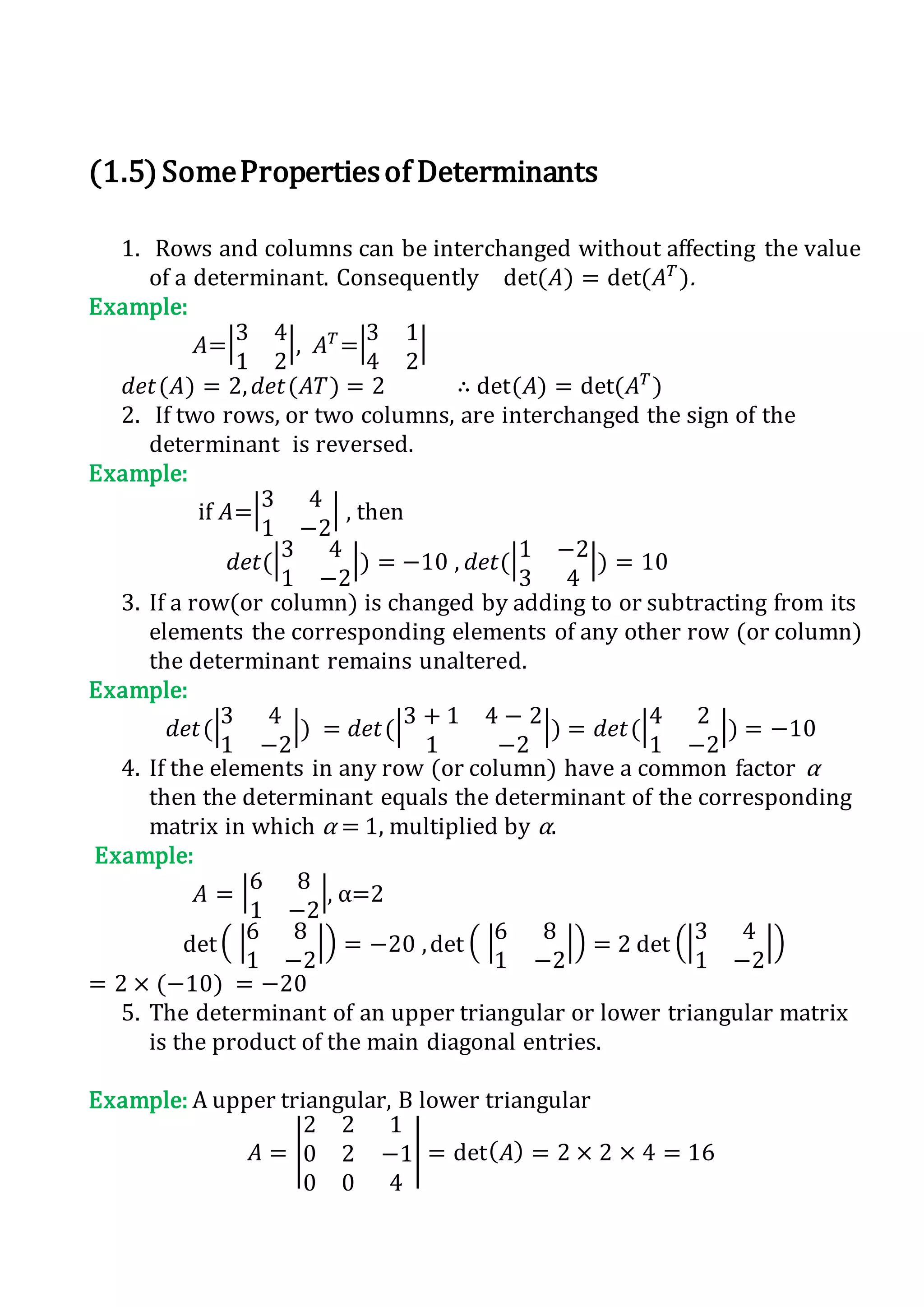
Example: cofactor expansion along the first column
𝐴=[
3 1 0
−2 −4 3
5 4 −2
] . evaluate 𝑑𝑒𝑡(𝐴) by cofactor expansion along the
column of 𝐴 .
𝑑𝑒𝑡(𝐴) = [
3 1 0
−2 −4 3
5 4 −2
]

35. =3|−4 3
4 −2
|+(-2) |1 0
4 −2
|+5| 1 0
−4 3
| =3(-
4)+(-2)(-2)+5(3)=6

36. CHAPTER TWO
System of Linear Equations
In this chapter we study the system of linear equation. Then we
illustrate using of matrices to solve system linear equation in terms of the
methods of Homogeneous Systems, Gaussian Elimination, Gauss-Jordan
Elimination and Cramer’s Rule
(2.1)LinearEquations
Definition:
Let 𝑎1 , . . . , 𝑎 𝑛, 𝑦 be elements of 𝑅, and let 𝑥1, . . . , 𝑥 𝑛 be unknowns
(also called variables or 𝒊𝒏𝒅𝒆𝒕𝒆𝒓𝒎𝒊𝒏𝒂𝒕𝒆𝒔). Then an equation of the form
𝑎1 𝑥1+ … + 𝑎 𝑛 𝑥 𝑛= y
is called a linear equation in 𝒏 unknowns (over 𝑅), the scalars 𝒂𝒊 are
called the coefficients ofthe unknowns , and 𝒚 is called the constant term
of the equation.
Example:
𝑥1+2𝑥1=5 𝑎1=1 , 𝑎2=2 , y=5 (This equation are linear )
But:
𝑥2
1+3√ 𝑥2 =5 (This equation is not linear)
Note: not all 𝒂 are zero .
Definition:
A linear equation in the two variables 𝑥1and 𝑥2 is an equation that can in
the form 𝑎1 𝑥1 +𝑎2 𝑥2=b
Where 𝑎1, 𝑎2 , and b are numbers, in general a linear equation in the 𝒏
variables 𝑥1, 𝑥2,…, 𝑥 𝑛is an equation that can be written in the form
𝑎1 𝑥1+𝑎2 𝑥2+…+𝑎 𝑛 𝑥 𝑛=𝑏
Where the coefficients 𝑎1, 𝑎2, …, 𝑎 𝑛 and the constant term 𝑏 are numbers.

37. Example: 𝑥1+7𝑥2=3 , 𝑥1+𝑥2+…+𝑥 𝑛=4
Some exampleof equations that are not linear are:
𝑥1
2
+𝑥1 𝑥3=3,
1
𝑥1
+𝑥2+𝑥3=
5
2
, 𝑒(𝑥1)
+𝑥2=
1
2
,
𝑥1+𝑥2
𝑥3+𝑥4
=𝑥5 + 7
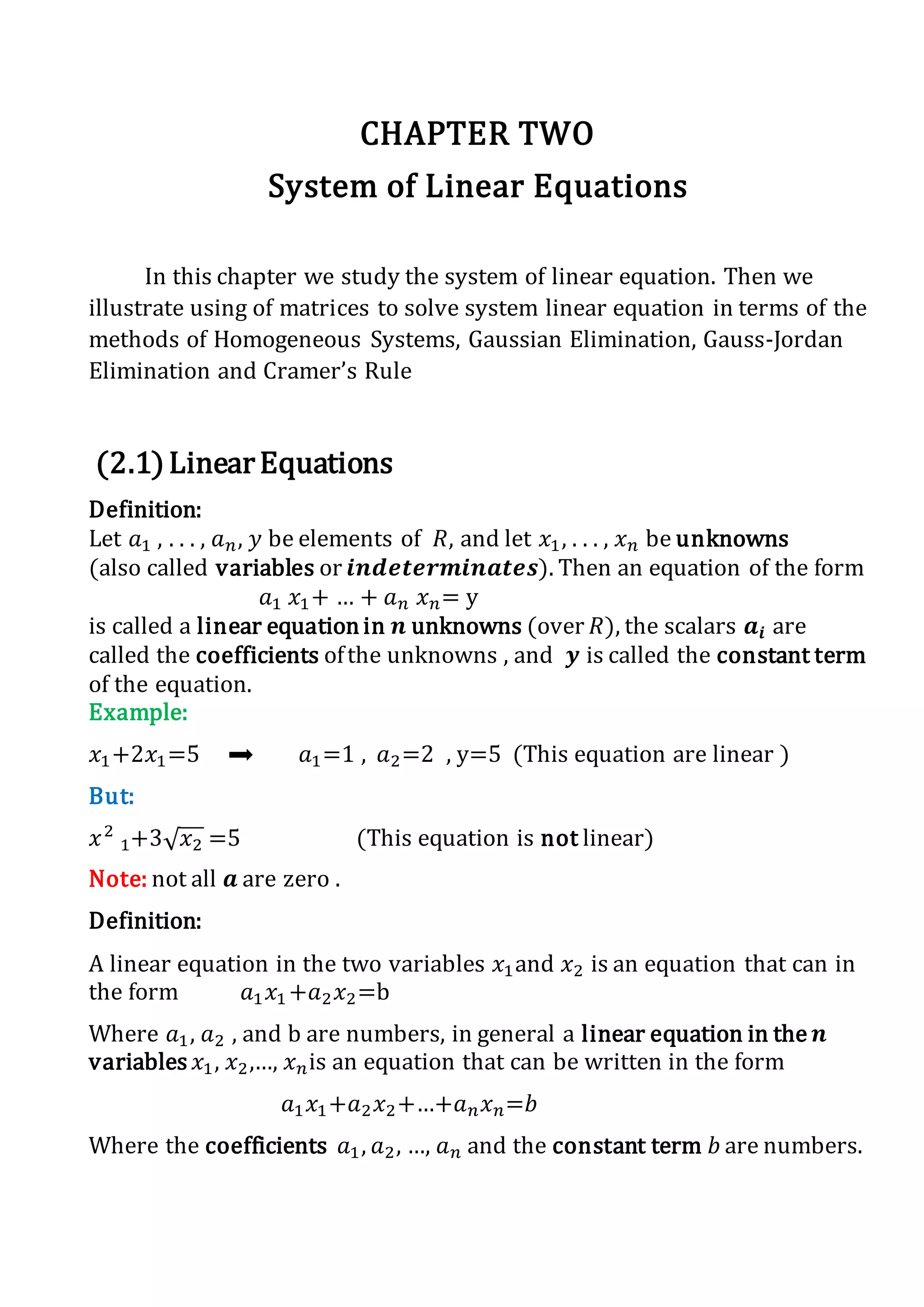
(2.2) LinearSystem
In general, a system of linear equations (also called a linear system) in
the variables 𝑥1 , 𝑥2, … , 𝑥 𝑛 consists of a finite number of linear
equations in these variables. The general form of a system of 𝑚 equations
in 𝑛 unknowns is
𝑎11 𝑥1 + 𝑎12 𝑥2 + ⋯ + 𝑎1𝑛 𝑥 𝑛 = 𝑏1
𝑎21 𝑥1 + 𝑎22 𝑥2 + ⋯ + 𝑎2𝑛 𝑥 𝑛 = 𝑏2
⋮ ⋮ ⋮ ⋮
𝑎 𝑚1 𝑥1 + 𝑎 𝑚2 𝑥2 + ⋯ + 𝑎 𝑚𝑛 𝑥 𝑛 = 𝑏𝑚
We will call such a system an 𝑚 × 𝑛 (𝑚 by 𝑛) linear system.
Example:
6𝑥1 + 2𝑥2 − 𝑥3 = 5
3𝑥1 + 𝑥2 − 4𝑥3 = 9
−𝑥1 + 3𝑥2 + 2𝑥3 = 0
Definition:
The coefficients of the variables form a matrix called the matrix of
coefficient of the system.
[
𝑎11 𝑎12 ⋯ 𝑎1𝑛
𝑎21 𝑎22 ⋯ 𝑎2𝑛
⋮ ⋮ ⋮
𝑎 𝑚1 𝑎 𝑚2 ⋯ 𝑎 𝑚𝑛
]
m×n

38. Definition:
The coefficients, together with the constant terms, form a matrix called
the augmented matrixof the system.
𝑎𝑢𝑔 𝐴=[
𝑎11 𝑎12 ⋯ 𝑎1𝑛 𝑦1
𝑎21 𝑎22 ⋯ 𝑎2𝑛 𝑦2
⋮ ⋮ ⋮ ⋮
𝑎 𝑚1 𝑎 𝑚2 ⋯ 𝑎 𝑚𝑛 𝑦 𝑛
]
m×n
Example: The matrix of coefficients and the augmented matrix of the
following system of linear equations are as shown:
𝑥1 + 𝑥2 + 𝑥3 = 2
2𝑥1 + 3𝑥2 + 𝑥3 = 3
𝑥1 − 𝑥2 − 2𝑥3 = −6
[
1 1 1
2 3 1
1 −1 −2
]
⏟
𝒎𝒂𝒕𝒓𝒊𝒙 𝒐𝒇 𝒄𝒐𝒆𝒇𝒇𝒊𝒄𝒊𝒆𝒏𝒕𝒔
[
1 1 1 2
2 3 1 3
1 −1 −2 −6
]
⏟
𝒂𝒖𝒈𝒎𝒆𝒏𝒕𝒆𝒅 𝒎𝒂𝒕𝒓𝒊𝒙
In solving systems of equations we are allowed to perform operations of
the following types:
1. Multiply an equation by a non-zero constant.
2. Add one equation (or a non-zero constant multiple of one equation) to
another equation.
These correspond to the following operations on the augmented matrix :
1. Multiply a row by a non-zero constant.
2. Add a multiple of one row to another row.
3. We also allow operations of the following type : Interchange two rows
in the matrix (this only amounts to writing down the equations of the
system in a different order).

39. Definition:
Operations of these three types are called Elementary Row Operations
(ERO's) on a matrix.
Example:
[
1 2 −1 5
3 1 −2 9
−1 4 2 0
]
𝑥 + 2𝑦 − 𝑧 = 5
3𝑥 + 𝑦 − 2𝑧 = 9
−𝑥 + 4𝑦 + 2𝑧 = 0
𝑅3 → 𝑅3 + 𝑅1 [
1 2 −1 5
3 1 −2 9
0 6 1 5
]
𝑥 + 2𝑦 − 𝑧 = 5
3𝑥 + 𝑦 − 2𝑧 = 9
6𝑦 + 𝑧 = 5
𝑅2 → 𝑅2 − 3𝑅1 [
1 2 −1 5
0 −5 1 −6
0 6 1 5
]
𝑥 + 2𝑦 − 𝑧 = 5
− 5𝑦 + 𝑧 = −6
6𝑦 + 𝑧 = 5
𝑅2 → 𝑅2 + 𝑅3 [
1 2 −1 5
0 1 2 −1
0 6 1 5
]
𝑥 + 2𝑦 − 𝑧 = 5
𝑦 + 2𝑧 = −1
6𝑦 + 𝑧 = 5
𝑅3 → 𝑅3 − 6𝑅2 [
1 2 −1 5
0 1 2 −1
0 0 −11 11
]
𝑥 + 2𝑦 − 𝑧 = 5
𝑦 + 2𝑧 = −1
− 11𝑧 = 11
𝑅3 × (−
1
11
) [
1 2 −1 5
0 1 2 −1
0 0 1 −1
]
𝑥 + 2𝑦 − 𝑧 = 5 … ( 𝐴)
𝑦 + 2𝑧 = −1 … ( 𝐵)
𝑧 = −1 … ( 𝐶)
We have produced a new system of equations, this is easily solved:

40. 𝐵𝑎𝑐𝑘𝑠𝑢𝑏𝑠𝑡𝑖𝑡𝑢𝑡𝑖𝑜𝑛
{
(C) z = −1
(B) y = −1 − 2z → y = −1 − 2(−1) = 1
( 𝐴) 𝑥 = 5 − 2𝑦 + 𝑧 → 𝑥 = 5 − 2(1) + (−1) = 2
∴ 𝑥 = 2, 𝑦 = 1, 𝑧 = −1
(2.2.1)HomogeneousSystems
A system of linear equations is said to be homogeneous if all the constant
terms are zeros, a system of homogeneous linear equations is a system of
the form
𝑎11 𝑥1 + 𝑎12 𝑥2 + ⋯ + 𝑎1𝑚 𝑥 𝑚 = 0
𝑎21 𝑥1 + 𝑎22 𝑥2 + ⋯ + 𝑎2𝑚 𝑥 𝑚 = 0
⋮ ⋮ ⋮ ⋮
𝑎 𝑛1 𝑥1 + 𝑎 𝑛2 𝑥2 + ⋯ + 𝑎 𝑛𝑚 𝑥 𝑚 = 0
Such a system is always consistent as 𝑥1 = 0, 𝑥2 = 0 , …. , 𝑥 𝑚 = 0is a
solution, this solution is called the trivial (or zero) solution, any other
solution is called a non-trivial solution.
Example:
𝑥 − 𝑦 = 0
𝑥 + 𝑦 = 0
Has only the trivial solution, whereas the homogeneous system
𝑥 − 𝑦 + 𝑧 = 0
𝑥 + 𝑦 + 𝑧 = 0
Has the complete solution 𝑥 = −𝑧; 𝑦 = 0; 𝑧 arbitrary. In particular,
taking 𝑧 = 1 gives the non-trivial solution
𝑥 = −1; 𝑦 = 0; 𝑧 = 1.
There is simple but fundamental theorem concerning homogeneous
systems.

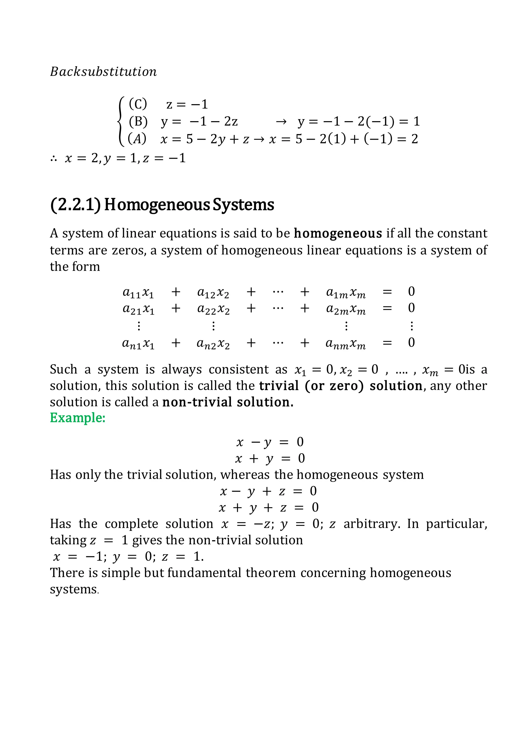
41. (2.2.2)GaussianElimination
This method is used to solve the linear system 𝐴𝑋 = 𝐵 by transforms the
augmented matrix [𝐴: 𝐵] to row echelon form and then uses substitution
to obtain the solution this procedure some what more efficient than
Gauss-Jordan reduction.
Consider a linear system
1. Construct the augmented matrix for the system.
2. Use elementary row operation to transform the augmented matrix
into a triangular one.
3. Write down the new linear system for which the triangular matrix is
the associated augmented matrix.
4. Solve the new system, you may need to assign some parametric
values to some unknowns, and then apply the method of back
substitution to solve the new system.
Example: We use Gaussian elimination to solve the system of linear
equations.
2𝑥2 + 𝑥3 = −8
𝑥1 − 2𝑥2 − 3𝑥3 = 0
−𝑥1 + 𝑥2 + 2𝑥3 = 3
The augmented matrix is
[
0 2 1 ⋮ −8
1 −2 −3 ⋮ 0
−1 1 2 ⋮ 3
]
Swap Row1 and Row2
[
1 −2 −3 ⋮ 0
0 2 1 ⋮ −8
−1 1 2 ⋮ 3
]
Add Row1 to Row3

42. [
1 −2 −3 ⋮ 0
0 2 1 ⋮ −8
0 −1 −1 ⋮ 3
]
Swap Row2 and to Row3
[
1 −2 −3 ⋮ 0
0 −1 −1 ⋮ 3
0 2 1 ⋮ −8
]
Add twice Row2 to Row3
[
1 −2 −3 ⋮ 0
0 −1 −1 ⋮ 3
0 0 −1 ⋮ −2
]
Multiply Row3 by -1
[
1 −2 −3 ⋮ 0
0 −1 −1 ⋮ 3
0 0 1 ⋮ 2
]
𝑥1 − 2𝑥2 − 3𝑥3 = 0…….(a)
−𝑥2 − 𝑥3 = 3……..(b)
𝑥3 = 2……..(c)
Then 𝑥3 = 2 and we put (c) in (b)
Then 𝑥2 = −5 and we put (b)and (c) in (a)
Then 𝑥1 =-4.
(2.2.3) Gauss-JordanElimination
The Gauss-Jordan elimination method to solve a system of linear
equations is described in the following steps.
1. Write the augmented matrix of the system.
2. Use row operations to transform the augmented matrix in the
form described below, which is called the reduced row echelon
form (RREF).

43. 3. Stop process in step 2 if you obtain a row whose elements are
all zeros except the last one on the right. In that case, the
system is inconsistent and has no solutions. Otherwise, finish
step 2 and read the solutions of the system from the final
matrix.
Note: When doing step 2, row operations can be performed in any order.
Try to choose row operations so that as few fractions as possible are
carried through the computation. This makes calculation
easier when working by hand.
Example: we Solve the following system by using the Gauss-Jordan
elimination method.
{
𝑥 + 𝑦 + 𝑧 = 5
2𝑥 + 3𝑦 + 5𝑧 = 8
4𝑥 + 5𝑧 = 2
The augmented matrix of the system is the following.
[
1 1 1 ⋮ 5
2 3 5 ⋮ 8
4 0 5 ⋮ 2
]
We will now perform row operations until we obtain a matrix in reduced
row echelon form.
[
1 1 1 ⋮ 5
2 3 5 ⋮ 8
4 0 5 ⋮ 2
]
R2−2R1
→ [
1 1 1 ⋮ 5
0 1 3 ⋮ −2
4 0 5 ⋮ 2
]
R3−4R1
→ [
1 1 1 ⋮ 5
0 1 3 ⋮ −2
0 −4 1 ⋮ −18
]
R3+4R2
→ [
1 1 1 ⋮ 5
0 1 3 ⋮ −2
0 0 13 ⋮ −26
]
1
13
R3
→ [
1 1 1 ⋮ 5
0 1 3 ⋮ −2
0 0 1 ⋮ −2
]
R2−3R3
→ [
1 1 1 ⋮ 5
0 1 0 ⋮ 4
0 0 1 ⋮ −2
]
R1−R3
→ [
1 1 0 ⋮ 7
0 1 0 ⋮ 4
0 0 1 ⋮ −2
]
R1−R2
→ [
1 0 0 ⋮ 3
0 1 0 ⋮ 4
0 0 1 ⋮ −2
]

44. From this final matrix, we can read the solution of the system. It is
𝑥 = 3, 𝑦 = 4, 𝑧 = −2.
(2.2.4) Cramer’sRule
If 𝐴𝑋 = 𝐵 is a system of linear equation in n-unknown, such that
𝑑𝑒𝑡(𝐴) ≠ 0 then the system has a unique solution, this solution is
𝑋1 =
𝑑𝑒𝑡(𝐴1 )
𝑑𝑒𝑡(𝐴)
, 𝑋2 =
𝑑𝑒𝑡(𝐴2)
𝑑𝑒𝑡(𝐴)
, 𝑋3 =
𝑑𝑒𝑡(𝐴3)
𝑑𝑒𝑡(𝐴)
Where 𝐴𝑖 is the matrix obtained by replacing the entries in the 𝑖 𝑡ℎ
column
of 𝐴 by the entries of 𝑏𝑡ℎ
column. The system
𝑎11 𝑥1 + 𝑎12 𝑥2 + ⋯ + 𝑎1𝑚 𝑥 𝑚 = 𝑏1
𝑎21 𝑥1 + 𝑎22 𝑥2 + ⋯ + 𝑎2𝑚 𝑥 𝑚 = 𝑏2
⋮ ⋮ ⋮ ⋮
𝑎 𝑛1 𝑥1 + 𝑎 𝑛2 𝑥2 + ⋯ + 𝑎 𝑛𝑚 𝑥 𝑚 = 𝑏𝑛
[
𝑎11 𝑎12 ⋯ 𝑎1𝑚 𝑏1
𝑎21 𝑎22 ⋯ 𝑎2𝑚 𝑏2
⋮ ⋮ ⋮ ⋮
𝑎 𝑛1 𝑎 𝑛2 ⋯ 𝑎 𝑛𝑚 𝑏 𝑛
]
n×m
A=[
𝑎11 𝑎12 ⋯ 𝑎1𝑚
𝑎21 𝑎22 ⋯ 𝑎2𝑚
⋮ ⋮ ⋮
𝑎 𝑛1 𝑎 𝑛2 ⋯ 𝑎 𝑛𝑚
]
n×m
𝐴1 = [
𝑏1 𝑎12 ⋯ 𝑎1𝑚
𝑏2 𝑎22 ⋯ 𝑎2𝑚
⋮ ⋮ ⋮
𝑏 𝑛 𝑎 𝑛2 ⋯ 𝑎 𝑛𝑚
]
n×m
, 𝐴2=[
𝑎11 𝑏1 ⋯ 𝑎1𝑚
𝑎21 𝑏2 ⋯ 𝑎2𝑚
⋮ ⋮ ⋮
𝑎 𝑛1 𝑏 𝑛 ⋯ 𝑎 𝑛𝑚
]
n×m
, … , 𝐴 𝑚=[
𝑎11 𝑎12 ⋯ 𝑏 𝑚
𝑎21 𝑎22 ⋯ 𝑏 𝑚
⋮ ⋮ ⋮
𝑎 𝑛1 𝑎 𝑛2 ⋯ 𝑏 𝑚
]
n×m

45. Example: we use crammer’s Rule to solve:
3𝑥1 + 4𝑥2 − 3𝑥3 = 5
3𝑥1 − 2𝑥2 + 4𝑥3 = 7
3𝑥1 + 2𝑥2 − 𝑥3 = 2
In matrix form 𝐴𝑋 = 𝑏 or [𝑎1 𝑎2 𝑎3 ]𝑋 = 𝑏 this is
[
3 4 −3
3 −2 4
3 2 −1
] [
𝑥1
𝑥2
𝑥3
] = [
5
7
3
].
Cramer’s Rule says that 𝑥1=
det(𝐴1)
det(𝐴)
, 𝑥2=
det(𝐴2)
det(𝐴)
, 𝑥3 =
det(𝐴3)
det(𝐴)
𝐴 = [
3 4 −3
3 −2 4
3 2 −1
] , 𝑑𝑒𝑡(𝐴) = 6
𝐴1 = [
5 4 −3
7 −2 4
3 2 −1
] , 𝑑𝑒𝑡(𝐴1 ) = −14
𝐴2 = [
3 5 −3
3 7 4
3 3 −1
] , 𝑑𝑒𝑡(𝐴2) = 54
𝐴3=[
3 4 5
3 −2 7
3 2 3
] , 𝑑𝑒𝑡(𝐴3) = 48
𝑥1 =
−14
6
= −
7
3
, 𝑥2 =
54
6
= 9 , 𝑥3 =
48
6
= 8.

46. 𝑹𝒆𝒇𝒆𝒓𝒆𝒏𝒄𝒆𝒔
1. Dennis M. Schneider, Manfred Steeg ,Frank H. Young.
Linear Algebra a Concrete Introduction. MacmillanCo.
Unites of America, 1982.
2. S. Barry and S. Davis, Essential Math. Skills,National Library
of Australia, 2002.
3. Garth Williams . Linear Algebra With Applications .
Jones And Bartlett , Canada , 2001.
4. P. Dawkins . Linear Algebra.
http://www.cs.cornell.edu/courses/cs485/2006sp/linalg_c
omplete.pdf