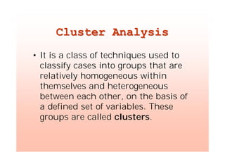
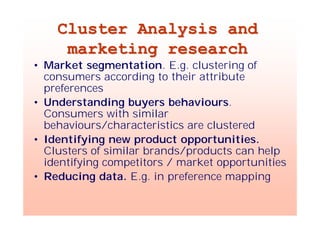
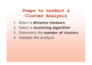
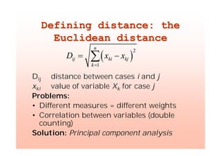
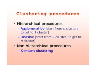
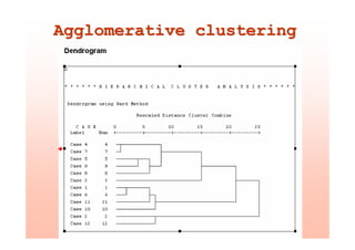
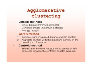
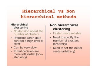
This document provides an overview of cluster analysis techniques. It defines cluster analysis as classifying cases into homogeneous groups based on a set of variables. The document then discusses how cluster analysis can be used in marketing research for market segmentation, understanding consumer behaviors, and identifying new product opportunities. It outlines the typical steps to conduct a cluster analysis, including selecting a distance measure and clustering algorithm, determining the number of clusters, and validating the analysis. Specific clustering methods like hierarchical, k-means, and deciding the number of clusters using the elbow rule are explained. The document concludes with an example of conducting a cluster analysis in SPSS.

1. SPSS TutorialSPSS Tutorial
AEB 37 / AE 802
Marketing Research Methods
Week 7

2. Cluster analysisCluster analysis
Lecture / Tutorial outline
• Cluster analysis
• Example of cluster analysis
• Work on the assignment

3. Cluster AnalysisCluster Analysis
• It is a class of techniques used to
classify cases into groups that are
relatively homogeneous within
themselves and heterogeneous
between each other, on the basis of
a defined set of variables. These
groups are called clusters.

4. Cluster Analysis andCluster Analysis and
marketing researchmarketing research
• Market segmentation. E.g. clustering of
consumers according to their attribute
preferences
• Understanding buyers behaviours.
Consumers with similar
behaviours/characteristics are clustered
• Identifying new product opportunities.
Clusters of similar brands/products can help
identifying competitors / market opportunities
• Reducing data. E.g. in preference mapping

5. Steps to conduct aSteps to conduct a
Cluster AnalysisCluster Analysis
1. Select a distance measure
2. Select a clustering algorithm
3. Determine the number of clusters
4. Validate the analysis

6. REGR factor score 2 for analysis 1
43210-1-2-3
REGRfactorscore1foranalysis1
3
2
1
0
-1
-2
-3
-4

7. Defining distance: theDefining distance: the
Euclidean distanceEuclidean distance
Dij distance between cases i and j
xki value of variable Xk for case j
Problems:
• Different measures = different weights
• Correlation between variables (double
counting)
Solution: Principal component analysis
 
2
1
n
ij ki kj
k
D x x

 

8. Clustering proceduresClustering procedures
• Hierarchical procedures
– Agglomerative (start from n clusters,
to get to 1 cluster)
– Divisive (start from 1 cluster, to get to
n cluster)
• Non hierarchical procedures
– K-means clustering

9. Agglomerative clusteringAgglomerative clustering

10. AgglomerativeAgglomerative
clusteringclustering
• Linkage methods
– Single linkage (minimum distance)
– Complete linkage (maximum distance)
– Average linkage
• Ward’s method
1. Compute sum of squared distances within clusters
2. Aggregate clusters with the minimum increase in the
overall sum of squares
• Centroid method
– The distance between two clusters is defined as the
difference between the centroids (cluster averages)

11. KK--means clusteringmeans clustering
1. The number k of cluster is fixed
2. An initial set of k “seeds” (aggregation centres) is
provided
• First k elements
• Other seeds
3. Given a certain treshold, all units are assigned to
the nearest cluster seed
4. New seeds are computed
5. Go back to step 3 until no reclassification is
necessary
Units can be reassigned in successive steps
(optimising partioning)

12. Hierarchical vs NonHierarchical vs Non
hierarchical methodshierarchical methods
Hierarchical
clustering
• No decision about the
number of clusters
• Problems when data
contain a high level of
error
• Can be very slow
• Initial decision are
more influential (one-
step only)
Non hierarchical
clustering
• Faster, more reliable
• Need to specify the
number of clusters
(arbitrary)
• Need to set the initial
seeds (arbitrary)

13. Suggested approachSuggested approach
1. First perform a hierarchical
method to define the number of
clusters
2. Then use the k-means procedure
to actually form the clusters

14. Defining the number ofDefining the number of
clusters: elbow rule (1)clusters: elbow rule (1)
Agglomeration Schedule
4 7 .015 0 0 4
6 10 .708 0 0 5
8 9 .974 0 0 4
4 8 1.042 1 3 6
1 6 1.100 0 2 7
4 5 3.680 4 0 7
1 4 3.492 5 6 8
1 11 6.744 7 0 9
1 2 8.276 8 0 10
1 12 8.787 9 0 11
1 3 11.403 10 0 0
Stage
1
2
3
4
5
6
7
8
9
10
11
Cluster 1Cluster 2
Cluster Combined
CoefficientsCluster 1 Cluster 2
Stage Cluster First
Appears
Next Stage
Stage Number of clusters
0 12
1 11
2 10
3 9
4 8
5 7
6 6
7 5
8 4
9 3
10 2
11 1
n

15. Elbow rule (2): theElbow rule (2): the
screescree diagramdiagram
0
2
4
6
8
10
12
11 10 9 8 7 6 5 4 3 2 1
Number of clusters
Distance

16. Validating theValidating the
analysisanalysis
• Impact of initial seeds / order of
cases
• Impact of the selected method
• Consider the relevance of the
chosen set of variables

17. SPSS ExampleSPSS Example

18. Component1
2.01.51.0.50.0-.5-1.0-1.5
Component2
1.5
1.0
.5
0.0
-.5
-1.0
-1.5
-2.0
LUCY
JULIA
FRED
ARTHUR
JENNIFER
THOMAS
MATTHEW
NICOLE
PAMELA
JOHN

19. Agglomeration Schedule
3 6 .026 0 0 8
2 5 .078 0 0 7
4 9 .224 0 0 5
1 7 .409 0 0 6
4 10 .849 3 0 8
1 8 1.456 4 0 7
1 2 4.503 6 2 9
3 4 9.878 1 5 9
1 3 18.000 7 8 0
Stage
1
2
3
4
5
6
7
8
9
Cluster 1 Cluster 2
Cluster Combined
Coefficients Cluster 1 Cluster 2
Stage Cluster First
Appears
Next Stage
Number of clusters: 10 – 6 = 4

20. Component1
2.01.51.0.50.0-.5-1.0-1.5
Component2
1.5
1.0
.5
0.0
-.5
-1.0
-1.5
-2.0
Cluster Number of Ca
4
3
2
1
LUCY
JULIA
FRED
ARTHUR
JENNIFER
THOMAS
MATTHEW
NICOLE
PAMELA
JOHN

21. Open the datasetOpen the dataset
supermarkets.savsupermarkets.sav
From your N: directory (if you saved it
there last time
Or download it from:
http://www.rdg.ac.uk/~aes02mm/
supermarket.sav
• Open it in SPSS

22. TheThe supermarkets.savsupermarkets.sav
datasetdataset

23. Run PrincipalRun Principal
Components AnalysisComponents Analysis
and save scoresand save scores
• Select the variables to perform the
analysis
• Set the rule to extract principal
components
• Give instruction to save the
principal components as new
variables

24. Cluster analysis:Cluster analysis:
basic stepsbasic steps
• Apply Ward’s methods on the
principal components score
• Check the agglomeration schedule
• Decide the number of clusters
• Apply the k-means method

25. Analyse / ClassifyAnalyse / Classify

26. Select the componentSelect the component
scoresscores
Select from here Untick this

27. Select WardSelect Ward’’s algorithms algorithm
Click here
first
Select
method here

28. Output: AgglomerationOutput: Agglomeration
scheduleschedule

29. Number of clustersNumber of clusters
Identify the step where the “distance coefficients” makes a bigger
jump

30. TheThe screescree diagramdiagram
(Excel needed)(Excel needed)
Distance
0
100
200
300
400
500
600
700
800
118
120
122
124
126
128
130
132
134
136
138
140
142
144
146
148
Step

31. Number of clustersNumber of clusters
Number of cases 150
Step of ‘elbow’ 144
__________________________________
Number of clusters 6

32. Now repeat theNow repeat the
analysisanalysis
• Choose the k-means technique
• Set 6 as the number of clusters
• Save cluster number for each case
• Run the analysis

33. KK--meansmeans

34. KK--means dialog boxmeans dialog box
Specify
number of
clusters

35. Save cluster membershipSave cluster membership
Click here
first Thick here

36. Final outputFinal output

37. Cluster membershipCluster membership

38. Component Matrixa
.810 -.294 -4.26E-02 .183 .173
.480 -.152 .347 .334 -5.95E-02
.525 -.206 -.475 -4.35E-02 .140
.192 -.345 -.127 .383 .199
.646 -.281 -.134 -.239 -.207
.536 .619 -.102 -.172 6.008E-02
.492 -.186 .190 .460 .342
1.784E-02 -9.24E-02 .647 -.287 .507
.649 .612 .135 -6.12E-02 -3.29E-03
.369 .663 .247 .184 1.694E-02
.124 -9.53E-02 .462 .232 -.529
2.989E-02 .406 -.349 .559 -8.14E-02
.443 -.271 .182 -5.61E-02 -.465
.908 -4.75E-02 -7.46E-02 -.197 -3.26E-02
.891 -5.64E-02 -6.73E-02 -.228 6.942E-04
Monthly amount spent
Meat expenditure
Fish expenditure
Vegetables expenditure
% spent in own-brand
product
Own a car
% spent in organic food
Vegetarian
Household Size
Number of kids
Weekly TV watching
(hours)
Weekly Radio listening
(hours)
Surf the web
Yearly household income
Age of respondent
1 2 3 4 5
Component
Extraction Method: Principal Component Analysis.
5 components extracted.a.
Component meaningComponent meaning
(tutorial week 5)(tutorial week 5)
1. “Old Rich Big
Spender” 3. Vegetarian TV
lover
4. Organic radio
listener
2. Family shopper
5. Vegetarian TV and
web hater

39. Final Cluster Centers
-1.34392 .21758 .13646 .77126 .40776 .72711
.38724 -.57755 -1.12759 .84536 .57109 -.58943
-.22215 -.09743 1.41343 .17812 1.05295 -1.39335
.15052 -.28837 -.30786 1.09055 -1.34106 .04972
.04886 -.93375 1.23631 -.11108 .31902 .87815
REGR factor score
1 for analysis 1
REGR factor score
2 for analysis 1
REGR factor score
3 for analysis 1
REGR factor score
4 for analysis 1
REGR factor score
5 for analysis 1
1 2 3 4 5 6
Cluster

40. Cluster interpretationCluster interpretation
through mean component valuesthrough mean component values
• Cluster 1 is very far from profile 1 (-1.34) and
more similar to profile 2 (0.38)
• Cluster 2 is very far from profile 5 (-0.93) and
not particularly similar to any profile
• Cluster 3 is extremely similar to profiles 3 and 5
and very far from profile 2
• Cluster 4 is similar to profiles 2 and 4
• Cluster 5 is very similar to profile 3 and very far
from profile 4
• Cluster 6 is very similar to profile 5 and very far
from profile 3

41. Which cluster toWhich cluster to
target?target?
• Objective: target the organic
consumer
• Which is the cluster that looks more
“organic”?
• Compute the descriptive statistics
on the original variables for that
cluster

42. Representation of factors 1Representation of factors 1
and 4and 4
(and cluster membership)(and cluster membership)
REGR factor score 1 for analysis 1
210-1-2-3
REGRfactorscore4foranalysis1
3
2
1
0
-1
-2
-3
Cluster Number of Ca
6
5
4
3
2
1