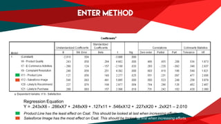
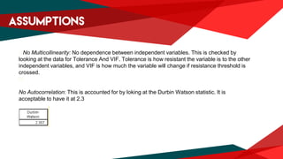
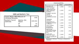
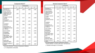
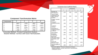
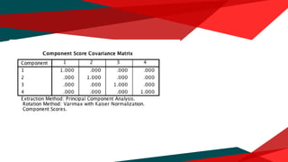
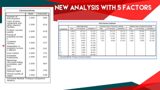
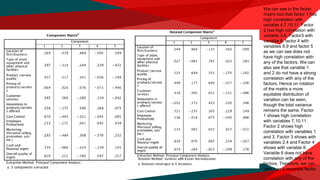
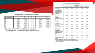
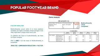
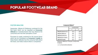
“
Aditya Banerjee 86
Amlan Anurag 90
Apoorva Jain 94
Boris Babu Joseph 98
Regression Equation
Y = .243xX6 - .286xX7 + .248xX9 + .127x11 + .546xX12 + .227xX20 + .2xX21 – 2.010
Product Line has the least effect on Csat. This should be looked at last when increasing efforts.
Salesforce Image has the most effect on Csat. This should be looked at first when increasing efforts.
Existence of Homoscedasticity: All errors have constant variance
This is tested by looking at scatter plots of each independent variable to the
dependent variable.
We see that x6, x12,
and x20 have mild
heteroscedasticity, but
this magnitude can be
ignored.
Functional Form of Regression is Linear: The highest power of the equation is
1, i.e. when plotted, the regression equation is a straight line.
Sphericity of Errors: All errors are normally distributed.
As can be seen, there is only one outlier when looking
at errors.
�No Multicollinearity: No dependence between independent variables. This is checked by
looking at the data for Tolerance And VIF. Tolerance is how resistant the variable is to the other
independent variables, and VIF is how much the variable will change if resistance threshold is
crossed.
�
No Autocorrelation: This is accounted for by loking at the Durbin Watson statistic. It is
acceptable to have it at 2.3
The R2 is .835, and the Adjusted R2 is .822. This shows that this
model is robust as it can be generalised for 82% of the population.
The SEE is also at .5027 which is advisable.
When efforts are being made to increase C Sat, the bulk of our efforts should be directed towards x12.
E Commerce activities show coefficient of -.268 which show that while there is an increase in e
commerce activities, it might not be contributing to increasing consumer satisfaction. Hence, work
needs to be done there in the form discounts, or other offers that can be put online
The highest correlation seen is between the variables cost control and cash and financial
management which is 0.496, which is not very strong.
“
To determine the number of clusters we put the condition of Eigen value>1. This gave us four factors. But as
we can see four factors are explaining only 58% of the variance which is below our agreeable limit. We can
also see that after 4 factors, each additional factor is explaining a very small amount of variation. Hence we
put 5 factors a priori and run the analysis again, the result of which can be seen below.
We can see in the factor
matrix box that factor 1 has
high correlation with
variable 4,7,10,11. Factor
2 has high correlation with
variable 3,5. Factor3 with
variable 6, factor 4 with
variables 8,9 and factor 5
as we can see does not
have high correlation with
any of the factors. We can
also see that variable 1
and 2 do not have a strong
correlation with any of the
factors. Hence on rotation
of the matrix a more
equitable distribution of
variation can be seen,
though the total variance
remains the same. Factor
1 shows high correlation
with variables 7,10,11.
Factor 2 shows high
correlation with variables 1
and 3. Factor 3 shows with
variables 2,4 and Factor 4
shows with variable 8.
Variable 6 does not have
correlation with any of the
factors. Therefore, we can
take it as a separate factor.
Taking the correlation of the variables with their
factors we have given the following labels to the
five factors extracted. :
1. Cost management
2. Product service
3. Pricing of machinery
4. Marketing
5. Employee productivity.
DATA CLEANING
We have converted the missing values in
the Likert scale (1-7) .
Values which were shown to be higher than 7 were
replaced with the mean of the given variable.
This produced a whole new set of variables for the
operation.
This was done using data transform.
TRANFORM > REPLACE MISSING VALUES
Select Data mean
CHANGE CAPTURED
Change from 9 to mean values for that particular variable.
FACTOR ANALYSIS
Multicollinearity occurs when 2 or more predictor
variables are highly correlated. Small changes in the
data might lead to large jumps due to this.
To address the issue of multicollinearity, we have
run factor analysis.
With a KMO > .6, the issue of Multicollinearity is
surpassed.
ANALYZE > DIMENSION REDUCTION > FACTOR
Multicollinearity
check
completed
FACTOR ANALYSIS
Awareness, Attitude & Preference combined for the
first factor which can be classified as Consumer
Attitude as it showed factors that may influence the
consumers and how their perception is built
Purchase & Loyalty combined for the second factor
which can be considered as Consumer Loyalty as
these factors reflected how the consumer feels about
the brand, and holds it above others in comparison.
CLUSTERING
The highest change in coefficient was noticed at
Stage 40 to Stage 41 which means that
agglomeration had to stop at this point.
N = 45
No. of Clusters = 45 – 40 = 4
PROFILING AND INTERPRETATION
Gender & Usage
Anova test was run to check if the classification was
significantly different when based on Gender or
Usage patterns.
It was found that no significant associations were
present for the same.
K MEANS VS HEIRARCHIAL CLUSTERING
It was found that there were major differences in the
number of cases/respondents that each cluster took
from the different methods used.
Although the number of clusters are same the mean
values for various variables will also differ
accordingly across the two methods due to the
change in respondents
Cluster 1 15
2 12
3 5
4 5
5 8
Valid 45
Missing 0
Hierarchical Method
K Means Method

Multivariate data analysis regression, cluster and factor analysis on spss

  • 1.
    “ Aditya Banerjee 86 AmlanAnurag 90 Apoorva Jain 94 Boris Babu Joseph 98
  • 3.
    Regression Equation Y =.243xX6 - .286xX7 + .248xX9 + .127x11 + .546xX12 + .227xX20 + .2xX21 – 2.010 Product Line has the least effect on Csat. This should be looked at last when increasing efforts. Salesforce Image has the most effect on Csat. This should be looked at first when increasing efforts.
  • 4.
    Existence of Homoscedasticity:All errors have constant variance This is tested by looking at scatter plots of each independent variable to the dependent variable. We see that x6, x12, and x20 have mild heteroscedasticity, but this magnitude can be ignored.
  • 5.
    Functional Form ofRegression is Linear: The highest power of the equation is 1, i.e. when plotted, the regression equation is a straight line.
  • 6.
    Sphericity of Errors:All errors are normally distributed. As can be seen, there is only one outlier when looking at errors.
  • 7.
    �No Multicollinearity: Nodependence between independent variables. This is checked by looking at the data for Tolerance And VIF. Tolerance is how resistant the variable is to the other independent variables, and VIF is how much the variable will change if resistance threshold is crossed. � No Autocorrelation: This is accounted for by loking at the Durbin Watson statistic. It is acceptable to have it at 2.3
  • 8.
    The R2 is.835, and the Adjusted R2 is .822. This shows that this model is robust as it can be generalised for 82% of the population. The SEE is also at .5027 which is advisable.
  • 9.
    When efforts arebeing made to increase C Sat, the bulk of our efforts should be directed towards x12. E Commerce activities show coefficient of -.268 which show that while there is an increase in e commerce activities, it might not be contributing to increasing consumer satisfaction. Hence, work needs to be done there in the form discounts, or other offers that can be put online
  • 10.
    The highest correlationseen is between the variables cost control and cash and financial management which is 0.496, which is not very strong.
  • 12.
    “ To determine thenumber of clusters we put the condition of Eigen value>1. This gave us four factors. But as we can see four factors are explaining only 58% of the variance which is below our agreeable limit. We can also see that after 4 factors, each additional factor is explaining a very small amount of variation. Hence we put 5 factors a priori and run the analysis again, the result of which can be seen below.
  • 17.
    We can seein the factor matrix box that factor 1 has high correlation with variable 4,7,10,11. Factor 2 has high correlation with variable 3,5. Factor3 with variable 6, factor 4 with variables 8,9 and factor 5 as we can see does not have high correlation with any of the factors. We can also see that variable 1 and 2 do not have a strong correlation with any of the factors. Hence on rotation of the matrix a more equitable distribution of variation can be seen, though the total variance remains the same. Factor 1 shows high correlation with variables 7,10,11. Factor 2 shows high correlation with variables 1 and 3. Factor 3 shows with variables 2,4 and Factor 4 shows with variable 8. Variable 6 does not have correlation with any of the factors. Therefore, we can take it as a separate factor.
  • 19.
    Taking the correlationof the variables with their factors we have given the following labels to the five factors extracted. : 1. Cost management 2. Product service 3. Pricing of machinery 4. Marketing 5. Employee productivity.
  • 20.
    DATA CLEANING We haveconverted the missing values in the Likert scale (1-7) . Values which were shown to be higher than 7 were replaced with the mean of the given variable. This produced a whole new set of variables for the operation. This was done using data transform. TRANFORM > REPLACE MISSING VALUES Select Data mean
  • 21.
    CHANGE CAPTURED Change from9 to mean values for that particular variable.
  • 22.
    FACTOR ANALYSIS Multicollinearity occurswhen 2 or more predictor variables are highly correlated. Small changes in the data might lead to large jumps due to this. To address the issue of multicollinearity, we have run factor analysis. With a KMO > .6, the issue of Multicollinearity is surpassed. ANALYZE > DIMENSION REDUCTION > FACTOR Multicollinearity check completed
  • 23.
    FACTOR ANALYSIS Awareness, Attitude& Preference combined for the first factor which can be classified as Consumer Attitude as it showed factors that may influence the consumers and how their perception is built Purchase & Loyalty combined for the second factor which can be considered as Consumer Loyalty as these factors reflected how the consumer feels about the brand, and holds it above others in comparison.
  • 24.
    CLUSTERING The highest changein coefficient was noticed at Stage 40 to Stage 41 which means that agglomeration had to stop at this point. N = 45 No. of Clusters = 45 – 40 = 4
  • 25.
    PROFILING AND INTERPRETATION Gender& Usage Anova test was run to check if the classification was significantly different when based on Gender or Usage patterns. It was found that no significant associations were present for the same.
  • 26.
    K MEANS VSHEIRARCHIAL CLUSTERING It was found that there were major differences in the number of cases/respondents that each cluster took from the different methods used. Although the number of clusters are same the mean values for various variables will also differ accordingly across the two methods due to the change in respondents Cluster 1 15 2 12 3 5 4 5 5 8 Valid 45 Missing 0 Hierarchical Method K Means Method