machine learning techniques

1. 1
Cluster Analysis: Basic Concepts and Methods
 Cluster Analysis: Basic Concepts
 Partitioning Methods
 Hierarchical Methods
 Evaluation of Clustering
1

2. 2
What is Cluster Analysis?
 Cluster: A collection of data objects
 similar (or related) to one another within the same group
 dissimilar (or unrelated) to the objects in other groups
 Cluster analysis (or clustering, data segmentation, …)
 Finding similarities between data according to the
characteristics found in the data and grouping similar
data objects into clusters
 Unsupervised learning: no predefined classes (i.e., learning
by observations vs. learning by examples: supervised)
 Typical applications
 As a stand-alone tool to get insight into data distribution
 As a preprocessing step for other algorithms

3. 3
Clustering for Data Understanding and
Applications
 Biology: taxonomy of living things: kingdom, phylum, class, order,
family, genus and species
 Information retrieval: document clustering
 Land use: Identification of areas of similar land use in an earth
observation database
 Marketing: Help marketers discover distinct groups in their customer
bases, and then use this knowledge to develop targeted marketing
programs
 City-planning: Identifying groups of houses according to their house
type, value, and geographical location
 Earth-quake studies: Observed earth quake epicenters should be
clustered along continent faults
 Climate: understanding earth climate, find patterns of atmospheric
and ocean
 Economic Science: market research

4. 4
Clustering as a Preprocessing Tool (Utility)
 Summarization:
 Preprocessing for regression, PCA, classification, and
association analysis
 Compression:
 Image processing: vector quantization
 Finding K-Nearest Neighbors
 Localizing search to one or a small number of clusters
 Outlier detection
 Outliers are often viewed as those “far away” from any
cluster

5. Quality: What Is Good Clustering?
 A good clustering method will produce high quality
clusters
 high intra-class
intra-class similarity: cohesive within clusters
 low inter-class
inter-class similarity: distinctive between clusters
 Quality of a clustering method depends on
 similarity measure used by the method
 its implementation, and
 Its ability to discover some or all of the hidden patterns
5

6. Measure the Quality of Clustering
 Dissimilarity/Similarity metric
 Similarity - expressed as distance function - d(i, j)
 Definitions of distance functions are different for
interval-scaled, boolean, categorical, ordinal ratio, and
vector variables
 Weights should be associated with different variables
based on applications and data semantics
 Quality of clustering:
 A separate “quality” function that measures the
“goodness” of a cluster.
 It is hard to define “similar enough” or “good enough”

Answer is typically highly subjective
6

7. Considerations for Cluster Analysis
 Partitioning criteria
 Single level vs. hierarchical partitioning (often, multi-level
hierarchical partitioning is desirable)
 Separation of clusters
 Exclusive (e.g., one customer belongs to only one region) vs.
non-exclusive (e.g., one document may belong to more than one
class)
 Similarity measure
 Distance-based (e.g., Euclidian, road network, vector) vs.
connectivity-based (e.g., density or contiguity)
 Clustering space
 Full space (often when low dimensional) vs. subspaces (often in
high-dimensional clustering)
7

8. Requirements and Challenges
 Scalability

Clustering all the data instead of only on samples
 Ability to deal with different types of attributes

Numerical, binary, categorical, ordinal, linked, and mixture of these
 Constraint-based clustering
 User may give inputs on constraints
 Use domain knowledge to determine input parameters
 Interpretability and usability
 Others
 Discovery of clusters with arbitrary shape

Ability to deal with noisy data
 Incremental clustering and insensitivity to input order

High dimensionality
8

9. Major Clustering Approaches (I)
 Partitioning approach:
 Construct various partitions and then evaluate them by some
criterion, e.g., minimizing the sum of square errors
 Typical methods: k-means, k-medoids, CLARANS
 Hierarchical approach:
 Create a hierarchical decomposition of the set of data (or objects)
using some criterion
 Typical methods: Diana, Agnes, BIRCH, CAMELEON
 Density-based approach:
 Based on connectivity and density functions
 Typical methods: DBSACN, OPTICS, DenClue
 Grid-based approach:
 based on a multiple-level granularity structure
 Typical methods: STING, WaveCluster, CLIQUE
9

10. Major Clustering Approaches (II)
 Model-based:
 A model is hypothesized for each of the clusters and tries to find
the best fit of that model to each other
 Typical methods: EM, SOM, COBWEB
 Frequent pattern-based:
 Based on the analysis of frequent patterns
 Typical methods: p-Cluster
 User-guided or constraint-based:
 Clustering by considering user-specified or application-specific
constraints
 Typical methods: COD (obstacles), constrained clustering
 Link-based clustering:
 Objects are often linked together in various ways
 Massive links can be used to cluster objects: SimRank, LinkClus
10

11. 11
Alternatives to Calculate the Distance between
Clusters
 Single link: smallest distance between an element in one cluster and an
element in the other, i.e., dis(Ki, Kj) = min(tip, tjq)
 Complete link: largest distance between an element in one cluster and
an element in the other, i.e., dis(Ki, Kj) = max(tip, tjq)
 Average: avg distance between an element in one cluster and an
element in the other, i.e., dis(Ki, Kj) = avg(tip, tjq)
 Centroid: distance between the centroids of two clusters, i.e., dis(Ki, Kj) =
dis(Ci, Cj)
 Medoid: distance between the medoids of two clusters, i.e., dis(Ki, Kj) =
dis(Mi, Mj)
 Medoid: one chosen, centrally located object in the cluster

12. 12
Centroid, Radius and Diameter of a
Cluster (for numerical data sets)
 Centroid: the “middle” of a cluster
 Radius: square root of average distance from any point of the
cluster to its centroid
 Diameter: square root of average mean squared distance between
all pairs of points in the cluster
N
t
N
i mi
m
C
)
(
1



N
m
c
mi
t
N
i
m
R
2
)
(
1




)
1
(
2
)
(
1
1







N
N
mj
t
mi
t
N
j
N
i
m
D

13. 13
Cluster Analysis: Basic Concepts and Methods
 Cluster Analysis: Basic Concepts
 Partitioning Methods
 Hierarchical Methods
 Evaluation of Clustering
13

14. Partitioning Algorithms: Basic Concept
 Partitioning method: Partitioning a database D of n objects into a set of
k clusters, such that the sum of squared distances is minimized (where
ci is the centroid or medoid of cluster Ci)
 Given k, find a partition of k clusters that optimizes the chosen
partitioning criterion
 Global optimal: exhaustively enumerate all partitions
 Heuristic methods: k-means and k-medoids algorithms
 k-means : Each cluster is represented by the center of the cluster
 k-medoids or PAM (Partition around medoids) : Each cluster is
represented by one of the objects in the cluster
2
1 )
( i
C
p
k
i c
p
E i



 

14

15. The K-Means Clustering Method
 Given k, the k-means algorithm is implemented in four
steps:
 Partition objects into k nonempty subsets, clusters, by
choosing k centroids(centroid is the center, i.e., mean
point, of the cluster) and assigning objects to the
nearest centroids
 Compute new centroids of the clusters of the current
partitioning
 Assign each object to the cluster with the nearest
centroid
 Go back to Step 2 when the assignment does not
change
15

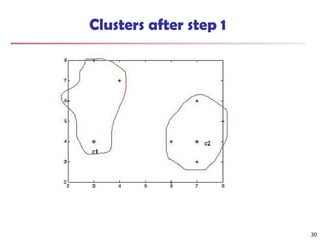
16. An Example of K-Means Clustering
K=2
Arbitrarily
choose k
objects as
centroids
and assign
each object
to nearest
centroid
Compute
new
centroids
for each
cluster
Update
the cluster
centroids
Reassign objects
Loop if
needed
16
The initial data
set

17. Example
 Suppose that the following items are given to
form cluster with k=2, using Manhattan distance
 {2,4,10,12,3,20,30,11,25}
 Initial centroids are 2 and 4.
17

18. Example
 When C1=2 and C2=4
 K1={2,3}, K2 = {4,10,12,20,30,11,25}
 When C1=2.5, C2=16
 K1={2,3,4}, K2 = {10,12,20,30,11,25}
18
C1 C2 K1 K2
3 18 {2,3,4,10} {12,20,30,11,25}
4.75 19.6 {2,3,4,10,11,12} {20,30,25}
7 25 {2,3,4,10,11,12} {20,30,25}

19. Exercise
 Suppose that the data mining task is to cluster
the following eight points into three clusters
A1(2,10), A2(2,5), A3(8,4), B1(5,8),
B2(7,5), B3(6,4), C1(1,2), C2(4,9)
 The distance is Euclidean distance.
 Let A1, B1, C1 be the initial centroids.
 Use K-mean algorithm to find the final three
clusters.
April 11, 2025 Data Mining: Concepts and Techniques 19

20. Comments on the K-Means Method
 Strength: Efficient: O(tkn), where n is # objects, k is # clusters, and t is #
iterations. Normally, k, t << n.

Comparing: PAM: O(k(n-k)2
)
 Comment: Often terminates at a local optimal.
 Weakness

Applicable only to objects in a continuous n-dimensional space

Using the k-modes method for categorical data

In comparison, k-medoids can be applied to a wide range of data

Need to specify k, the number of clusters, in advance (there are
ways to automatically determine the best k
 Sensitive to noisy data and outliers
 Not suitable to discover clusters with non-convex shapes
20

21. Variations of the K-Means Method
 Most of the variants of the k-means which differ in
 Selection of the initial k means
 Dissimilarity calculations
 Strategies to calculate cluster means
 Handling categorical data: k-modes
 Replacing means of clusters with modes
 Using new dissimilarity measures to deal with categorical objects
 Using a frequency-based method to update modes of clusters
 A mixture of categorical and numerical data: k-prototype method
21

22. What Is the Problem of the K-Means Method?
 The k-means algorithm is sensitive to outliers !
 Since an object with an extremely large value may substantially
distort the distribution of the data
 K-Medoids: Instead of taking the mean value of the object in a cluster
as a reference point, medoids can be used, which is the most
centrally located object in a cluster
0
1
2
3
4
5
6
7
8
9
10
0 1 2 3 4 5 6 7 8 9 10
0
1
2
3
4
5
6
7
8
9
10
0 1 2 3 4 5 6 7 8 9 10
22

23. 23
PAM: A Typical K-Medoids Algorithm
0
1
2
3
4
5
6
7
8
9
10
0 1 2 3 4 5 6 7 8 9 10
Total Cost = 20
0
1
2
3
4
5
6
7
8
9
10
0 1 2 3 4 5 6 7 8 9 10
K=2
Arbitrar
y choose
k object
as initial
medoids
0
1
2
3
4
5
6
7
8
9
10
0 1 2 3 4 5 6 7 8 9 10
Assign
each
remaini
ng
object to
nearest
medoids
Randomly select a
nonmedoid
object,Oramdom
Compute
total cost
of
swapping
0
1
2
3
4
5
6
7
8
9
10
0 1 2 3 4 5 6 7 8 9 10
Total Cost = 26
Swapping O
and Oramdom
If quality is
improved.
Do loop
Until no
change
0
1
2
3
4
5
6
7
8
9
10
0 1 2 3 4 5 6 7 8 9 10

24. The K-Medoid Clustering Method
 K-Medoids Clustering: Find representative objects (medoids) in clusters

PAM (Partitioning Around Medoids)

Starts from an initial set of medoids and iteratively replaces one
of the medoids by one of the non-medoids if it improves the total
distance of the resulting clustering

PAM works effectively for small data sets, but does not scale well
for large data sets (due to the computational complexity)
 Efficiency improvement on PAM

CLARA: PAM on samples
 CLARANS: Randomized re-sampling
24

25. Partitioning Around Medoids (PAM) algorithm
 Initialize: randomly select k of the n data points as the
medoids
 Associate each data point to the closest medoid. ("closest"
here is defined using any valid distance metric, most
commonly Euclidean distance, Manhattan distance or
Minkowski distance)
 For each medoid m
 For each non-medoid data point o

Swap m and o and compute the total cost of the
configuration
 Select the configuration with the lowest cost.
 Repeat steps 2 to 5 until there is no change in the medoid.
25

26. Example
ID X Y
X1 2 6
X2 3 4
X3 3 8
X4 4 7
X5 6 2
X6 6 4
X7 7 3
X8 7 4
X9 8 5
X10 7 6
26
Consider two clusters
k=2
Let C1 = (3,4),C2 =(7,4)
*
*

27. Distribution of data
27

28. 28
Xi Dist. from
C1=(3,4)
Dist. from
C2=(7,4)
Cluster
(2,6) 3 7 C1
(3,8) 4 8 C1
(4,7) 4 6 C1
(6,2) 5 3 C2
(6,4) 3 1 C2
(7,3) 5 1 C2
(8,5) 6 2 C2
(7,6) 6 2 C2
Manhattan Distance

29. 29

30. Clusters after step 1
30

31.  Selection of non-medoid point O’ randomly
 Assume O’ = (7,3)
31
Xi Dist. from
C1=(3,4)
Dist. from
C2=(7,4)
Dist. From
O’=(7,3)
(2,6) 3 7 8
(3,8) 4 8 9
(4,7) 4 6 7
(6,2) 5 3 2
(6,4) 3 1 2
(7,3) 5 1 1
(8,5) 6 2 3
(7,6) 6 2 3
Step 2

32. Clusters after step 2
32

33. Cost of Swapping
 Total cost = 3+4+4+2+2+1+3+3
= 22
 Cost of swapping medoid from c2 to O’ is
 S = current total cost – past total cost
= 22-20 = 2
 So, moving to O’ is bad and the previous choice
was good and algorithm terminates.
33

34. 34
Cluster Analysis: Basic Concepts and Methods
 Cluster Analysis: Basic Concepts
 Partitioning Methods
 Hierarchical Methods
 Evaluation of Clustering
34

35. Hierarchical Clustering
 Create a hierarchical decomposition of the set of data (or
objects) using some criterion
 Typical methods: Diana, Agnes, BIRCH, CHAMELEON
Step 0 Step 1 Step 2 Step 3 Step 4
b
d
c
e
a
a b
d e
c d e
a b c d e
Step 4 Step 3 Step 2 Step 1 Step 0
agglomerative
(AGNES)
divisive
(DIANA)
35

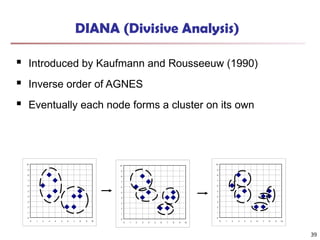
36. AGNES (Agglomerative Nesting)
 Introduced by Kaufmann and Rousseeuw (1990)
 Use the single-link method and the dissimilarity matrix
 Merge nodes that have the least dissimilarity
 Go on in a non-descending fashion
 Eventually all nodes belong to the same cluster
0
1
2
3
4
5
6
7
8
9
10
0 1 2 3 4 5 6 7 8 9 10
0
1
2
3
4
5
6
7
8
9
10
0 1 2 3 4 5 6 7 8 9 10
0
1
2
3
4
5
6
7
8
9
10
0 1 2 3 4 5 6 7 8 9 10
36

37. Dendrogram
 Decompose data objects into a several
levels of nested partitioning (tree of
clusters), called a dendrogram
 A clustering of the data objects is obtained
by cutting the dendrogram at the desired
level, then each connected component
forms a cluster
37

38. Dendrogram: Shows How Clusters are Merged
38

39. DIANA (Divisive Analysis)
 Introduced by Kaufmann and Rousseeuw (1990)
 Inverse order of AGNES
 Eventually each node forms a cluster on its own
0
1
2
3
4
5
6
7
8
9
10
0 1 2 3 4 5 6 7 8 9 10
0
1
2
3
4
5
6
7
8
9
10
0 1 2 3 4 5 6 7 8 9 10
0
1
2
3
4
5
6
7
8
9
10
0 1 2 3 4 5 6 7 8 9 10
39

40. Distance Matrix
 Given data values {7,10,20,28,35}
7 10 20 28 35
7 0
10 3 0
20 13 10 0
28 21 18 8 0
35 28 25 15 7 0

41. Agglomerative Clustering (Single
Linkage)
 Given data values {7,10,20,28,35}
7 10 20 28 35
7 0
10 3 0
20 13 10 0
28 21 18 8 0
35 28 25 15 7 0
Select Min Distance value and Form Single
Cluster with the corresponding Data Points

42. Agglomerative Clustering (Single
Linkage)
 Given data values {7,10,20,28,35}
(7,10) 20 28 35
(7,10) 0
20 10 0
28 18 8 0
35 25 15 7 0
Min of D(7,20)&D(10,20)
Min of D(7,28)&D(10,28)
Min of D(7,35)&D(10,35)

43. Agglomerative Clustering (Single
Linkage)
 Given data values {7,10,20,28,35}
(7,10) 20 (28,35)
(7,10) 0
20 10 0
(28,35) 18 8 0
Cluster 1 = {7,10}
Cluster 2 = {20,28,35}

44. Dendrogram
8
7
3
* * * * *
7 10 20 28 35

45. Agglomerative Clustering (Complete
Linkage)
 Given data values {7,10,20,28,35}
7 10 20 28 35
7 0
10 3 0
20 13 10 0
28 21 18 8 0
35 28 25 15 7 0
Select Min Distance value and Form Single
Cluster with the corresponding Data Points

46. Agglomerative Clustering (Complete
Linkage)
 Given data values {7,10,20,28,35}
(7,10) 20 28 35
(7,10) 0
20 13 0
28 21 8 0
35 28 15 7 0
Max of D(7,20)&D(10,20)
Max of D(7,28)&D(10,28)
Max of D(7,35)&D(10,35)

47. Agglomerative Clustering (Complete
Linkage)
 Given data values {7,10,20,28,35}
(7,10) 20 (28,35)
(7,10) 0
20 13 0
(28,35) 28 15 0
Cluster 1 = {7,10,20}
Cluster 2 = {28,35}

48. Example of Complete Linkage
Clustering
Distance
Matrix

49. Iteration 1
Using complete linkage clustering, the distance between (3,5)
and every other item is the maximum of the distance between
item and 3 and item 5.
(3,5) 1 2 4
(3,5) 0
1 11 0
2 10 9 0
4 9 6 5 0

50. After Iteration 3

51. For Single Linkage Dendrogram

52. Determining clusters
 One of the problems with hierarchical clustering is that
there is no objective way to say how many clusters there
are.
 Cutting the single linkage tree at the point shown below,
there will be two clusters

53. If the tree is cut as given below, than there will be one cluster
and two singletons.

54. Extensions to Hierarchical Clustering
 Major weakness of agglomerative clustering methods

Can never undo what was done previously

Do not scale well: time complexity of at least O(n2
), where
n is the number of total objects
 Integration of hierarchical & distance-based clustering

BIRCH (1996): uses CF(Clustering Features)-tree and
incrementally adjusts the quality of sub-clusters

CHAMELEON (1999): hierarchical clustering using
dynamic modeling
54

55. 55
Cluster Analysis: Basic Concepts and Methods
 Cluster Analysis: Basic Concepts
 Partitioning Methods
 Hierarchical Methods
 Evaluation of Clustering
55

56. Determine the Number of Clusters
 Empirical method
 # of clusters ≈√n/2 for a dataset of n points.
 Each cluster ≈√n points
 Elbow method
 For every value of K, calculate the within-cluster sum of squares (WCSS-
sum of square distances between the centroids and each points) value.
 Plot a graph of k versus their WCSS value. The graph will look like an elbow
 Use the turning point in the curve, where the graph starts to look like a
straight line, as the K value.
56

57. Determine the Number of Clusters
57
 Cross validation method
 Divide the given data set into m parts
 Use m – 1 parts to obtain a clustering model
 Use the remaining part to test the quality of the clustering

E.g., For each point in the test set, find the closest centroid,
and use the sum of squared distance between all points in the
test set and the closest centroids to measure how well the
model fits the test set
 For any k > 0, repeat it m times, compare the overall quality
measure w.r.t. different k’s, and find # of clusters that fits the data
the best

58. Measuring Clustering Quality
 Two methods: extrinsic vs. intrinsic
 Extrinsic: supervised, i.e., the ground truth (Ideal clustering
build using human experts) is available
 Compare the clustering against the ground truth using certain
clustering quality measure
 Ex. BCubed precision and BCubed recall metrics
 Intrinsic: unsupervised, i.e., the ground truth is unavailable
 Evaluate the goodness of a clustering by considering how
well the clusters are separated, and how compact the
clusters are.
 Ex. Silhouette coefficient
58

59. Measuring Clustering Quality: Extrinsic Methods
 Clustering quality measure: Q(C, Cg), for a clustering C given the
ground truth Cg.
 Q is good if it satisfies the following 4 essential criteria

Cluster homogeneity: pure the clusters, better the clustering
 Purity : Number of correctly matched class and cluster labels divided by
the number of total data points.

Cluster completeness: should assign objects belong to the
same category in the ground truth to the same cluster
 Rag bag: putting a heterogeneous object into a pure cluster
should be penalized more than putting it into a rag bag (i.e.,
“miscellaneous” or “other” category)

Small cluster preservation: splitting a small category into
pieces is more harmful than splitting a large category into
pieces
59