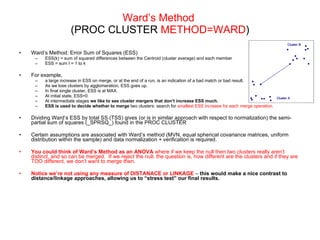
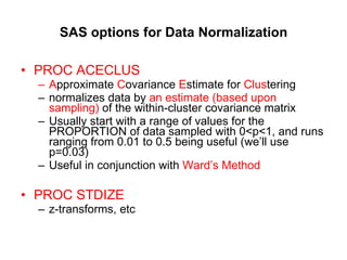
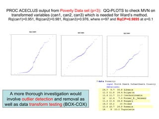
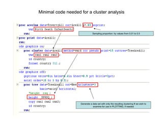
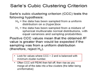
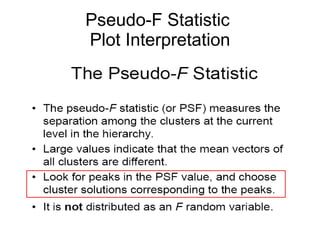
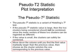
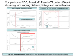
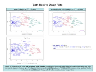
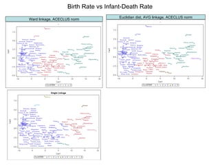
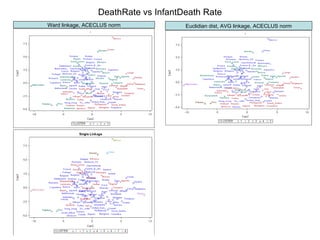
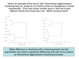
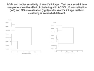
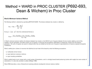
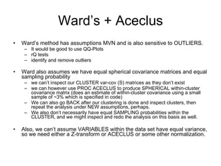
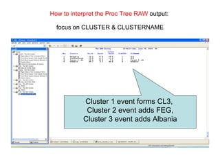
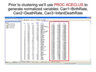
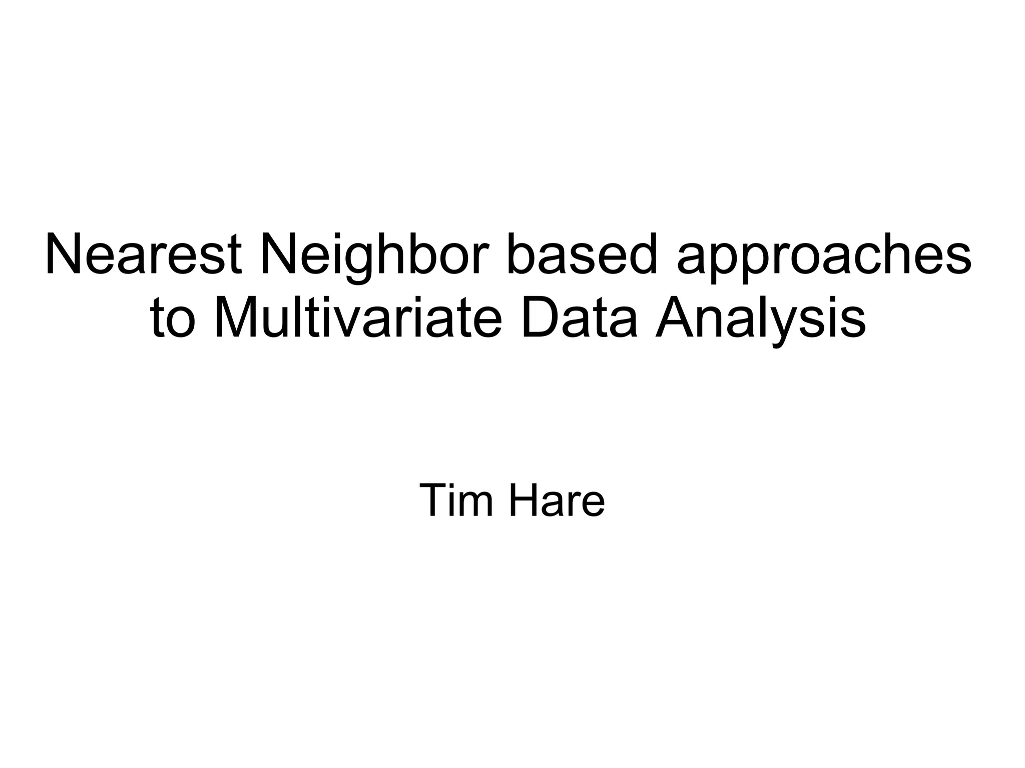
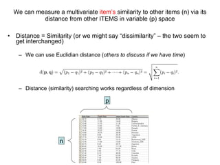
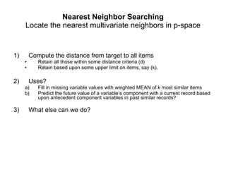
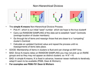
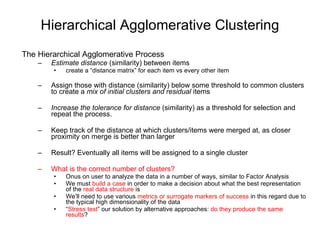
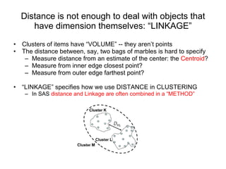
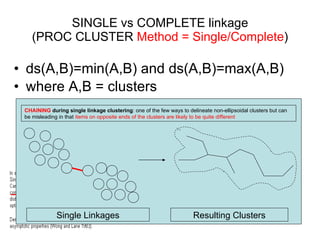
This document discusses different approaches to multivariate data analysis and clustering, including nearest neighbor methods, hierarchical clustering, and k-means clustering. It provides examples of using Ward's method, average linkage, and k-means clustering on poverty data to identify potential clusters of countries based on variables like birth rate, death rate, and infant mortality rate. Key lessons are that different linkage methods, distance measures, and data normalizations should be tested and that higher-dimensional data may require different variable spaces or transformations to identify meaningful clusters.

1. Nearest Neighbor based approaches to Multivariate Data Analysis Tim Hare

2. We can measure a multivariate item’s similarity to other items (n) via its distance from other ITEMS in variable (p) space Distance = Similarity (or we might say “dissimilarity” – the two seem to get interchanged) We can use Euclidian distance ( others to discuss if we have time ) Distance (similarity) searching works regardless of dimension p n

3. Nearest Neighbor Searching Locate the nearest multivariate neighbors in p-space Compute the distance from target to all items Retain all those within some distance criteria (d) Retain based upon some upper limit on items, say (k). Uses? Fill in missing variable values with weighted MEAN of k most similar items Predict the future value of a variable’s component with a current record based upon antecedent component variables in past similar records? What else can we do?

4. Clustering Approaches Hierarchical Clustering: Agglomerative OR Divisive we can group items (where distance = similarity) we can group variables (where correlation = similarity) Can use correlation coefficients for continuous random variables Can use Binary Weighting Schemes for presence of absence of certain characteristics (0,1 component values of item vector) See P674-678 Dean & Wichern Non-Hierarchical Clustering Divisive only (?) we group items only (where distance = similarity) . Statistical Clustering More recent Based on density estimates and mixed density estimation SAS appears to have a non-parmetric density estimate based clustering via MODECLUS. Parametric density estimate based clustering is discussed in Dean and Wichern (Section 12.5) R-language appears to offer parametric density estimate based statistical clustering via MCLUST (P705).

5. Non-Hierarchical Divisive The simple K-means Non-Hierarchical Divisive Process Pick K*, which is our initial “seed” number which we hope is the true cluster# Carry out RANDOM SAMPLING of the data set to establish “seed” Centroids (average location of cluster members) Go through list of items and reassign those that are closer to a “competing” cluster’s Centroid Calculate an updated Centroid value and repeat the process until no reassignments of items take place. GOOD: Membership of items in clusters is fluid and can change at ANY time. BAD: Since K-means relies on RANDOM SAMPLING you may not pick up on RARE groups and so they may not appear as distinct clusters: so  K* < K BAD: In simple K-means, K is fixed in advance, however newer methods to iteratively adapt K seem to be available (P696, Dean & Wichern). For examples see P696-701 Dean & Wichern

6. Hierarchical Agglomerative Clustering The Hierarchical Agglomerative Process Estimate distance (similarity) between items create a “distance matrix” for each item vs every other item Assign those with distance (similarity) below some threshold to common clusters to create a mix of initial clusters and residual items Increase the tolerance for distance (similarity) as a threshold for selection and repeat the process. Keep track of the distance at which clusters/items were merged at, as closer proximity on merge is better than larger Result? Eventually all items will be assigned to a single cluster What is the correct number of clusters? Onus on user to analyze the data in a number of ways, similar to Factor Analysis We must build a case in order to make a decision about what the best representation of the real data structure is We’ll need to use various metrics or surrogate markers of success in this regard due to the typical high dimensionality of the data “ Stress test ” our solution by alternative approaches: do they produce the same results ?

7. Distance is not enough to deal with objects that have dimension themselves: “LINKAGE” Clusters of items have “VOLUME” -- they aren’t points The distance between, say, two bags of marbles is hard to specify Measure distance from an estimate of the center: the Centroid ? Measure from inner edge closest point? Measure from outer edge farthest point? “ LINKAGE” specifies how we use DISTANCE in CLUSTERING In SAS distance and Linkage are often combined in a “METHOD”

8. SINGLE vs COMPLETE linkage (PROC CLUSTER Method = Single/Complete ) ds(A,B)=min(A,B) and ds(A,B)=max(A,B) where A,B = clusters min(S,Q)= max(S,Q)= CHAINING during single linkage clustering : one of the few ways to delineate non-ellipsoidal clusters but can be misleading in that items on opposite ends of the clusters are likely to be quite different Resulting Clusters Single Linkages

9. AVERAGE linkage (PROC CLUSTER Method = AVERAGE) Σ [MxN d(a i ,b i )]/ (MxN) As one would expect, less influenced by outliers than SINLGLE or COMPLETE [ d(A1,B1),d(A1,B2),d(A1,B3) d(A2,B1),d(A2,B2),d(A2,B3) d(A3,B1),d(A3,B2),d(A3,B3) ]/9

10. Ward’s Method (PROC CLUSTER METHOD=WARD ) Ward’s Method: Error Sum of Squares (ESS) ESS(k) = sum of squared differences between the Centroid (cluster average) and each member ESS = sum I = 1 to k For example, a large increase in ESS on merge, or at the end of a run, is an indication of a bad match or bad result. As we lose clusters by agglomeration, ESS goes up. In final single cluster, ESS is at MAX. At initial state, ESS=0 At intermediate stages we like to see cluster mergers that don’t increase ESS much. ESS is used to decide whether to merge two clusters: search for smallest ESS increase for each merge operation. Dividing Ward’s ESS by total SS (TSS) gives (or is in similar approach with respect to normalization) the semi-partial sum of squares (_SPRSQ_) found in the PROC CLUSTER Certain assumptions are associated with Ward’s method (MVN, equal spherical covariance matrices, uniform distribution within the sample) and data normalization + verification is required. You could think of Ward’s Method as an ANOVA where if we keep the null then two clusters really aren’t distinct, and so can be merged. If we reject the null, the question is, how different are the clusters and if they are TOO different, we don’t want to merge then. Notice we’re not using any measure of DISTANACE or LINKAGE – this would make a nice contrast to distance/linkage approaches, allowing us to “stress test” our final results.

11. SAS options for Data Normalization PROC ACECLUS A pproximate C ovariance E stimate for Clus tering normalizes data by an estimate (based upon sampling) of the within-cluster covariance matrix Usually start with a range of values for the PROPORTION of data sampled with 0<p<1, and runs ranging from 0.01 to 0.5 being useful (we’ll use p=0.03) Useful in conjunction with Ward’s Method PROC STDIZE z-transforms, etc

12. PROC ACECLUS output from Poverty Data set (p=3) : QQ-PLOTS to check MVN on transformed variables (can1, can2, can3) which is needed for Ward’s method. Rq(can1)=0.951, Rq(can2)=0.981, Rq(can3)=0.976, where n=97 and RqCP=0.9895 at α =0.1 A more thorough investigation would involve outlier detection and removal as well as data transform testing (BOX-COX)

13. Minimal code needed for a cluster analysis Generate a data set with only the resulting clustering # we wish to examine for use in PLOTTING, if needed Sampling proportion: try values from 0.01 to 0.5

14. PROC TREE output: how many clusters do we think are appropriate? (Distance criteria and value at time of merger on horizontal axis) Ward’s ? Average

16. Pseudo-F Statistic Plot Interpretation

17. Pseudo-T2 Statistic Plot Interpretation

18. Comparison of CCC, Pseudo-F, Pseudo-T2 under different clustering runs varying distance, linkage and normalization If we didn’t have a low dimensional variable set (p=3) it would be impossible to build a case on AVERAGE- and SIMPLE linkage Euclidian Dist, AVG linkage, Aceclus Normalized ? Ward Linkage, Aceclus Normalized What we want to see. Simple Linkage, Aceclus Normalized ?

19. Birth Rate vs Death Rate Notice the evidence for the known bias in Ward to equal numbers of observations per cluster where as with AVG the process allows us to have some small clusters in the lower right. The Expected Maximum Likelihood (EML) method in PROC CLUSTER produces similar results to Ward’s method, but with a slight bias in the opposite direction toward clusters of unequal sizes. Ward linkage, ACECLUS norm Euclidian dist, AVG linkage, ACECLUS norm

20. Birth Rate vs Infant-Death Rate Ward linkage, ACECLUS norm Euclidian dist, AVG linkage, ACECLUS norm

21. DeathRate vs InfantDeath Rate Ward linkage, ACECLUS norm Euclidian dist, AVG linkage, ACECLUS norm

22. Lessons learned? Since we used a low variable data set we can judge our success to some degree: But how would it be with a dimension p=20? CCC, Pseudo-F, and Pseudo-T2 critical Try different linkage/distance approaches Try different normalization approaches Consider the possibility that your data may need more variable space to be clustered, or different variable space: our particular p=3 were sufficient here to distinguish countries, but perhaps other/additional variables would allow better clustering? Could use +/- PCA in advance of clustering, perhaps? Keep in mind that certain methods have certain ASSUMPTIONS : example – Ward’s method has MVN density distribution mixture as an assumption, along with others. It was necessary to use appropriate normalization (ACECLUS) and verification to speak to these assumptions. These appear to be “diffuse, poorly differentiated” clusters, & we had our only real success with Ward’s Method in that we would NOT have been able to interpret higher dimensional data in the other instances via the critical metrics CCC, Pseudo-F, and Pseudo-T2 That said, the result appears to be stable across two very different clustering approaches (Ward’s Method, and Average Linkage) so that’s encouraging. Yet we would not KNOW this from the CCC, Pseudo-F, and Pseudo-T2 alone!

23. Q & A

24. Here’s an example of the risk of “bad” Hierarchical Agglomerative clustering early on: small run on 8 items shows us divergence in cluster membership. If the final cluster number were 4, then we’d have different results from these two runs. Which would be best? Slight difference in clustering with a robust approach but bad approaches can result in significant differences that will not be undone as Hierarchical Agglomerative clustering proceeds.

25. MVN and outlier sensitivity of Ward’s linkage: Test on a small 4 item sample to show the effect of clustering with ACECLUS normalization (left) and NO normalization (right) under Ward’s linkage method: clustering is somewhat different.

26. Method = WARD in PROC CLUSTER (P692-693, Dean & Wichern) in Proc Cluster

27. Ward’s + Aceclus Ward’s method has assumptions MVN and is also sensitive to OUTLIERS. It would be good to use QQ-Plots rQ tests identify and remove outliers Ward also assumes we have equal spherical covariance matrices and equal sampling probability we can’t inspect our CLUSTER var-cov (S) matrices as they don’t exist we can however use PROC ACECLUS to produce SPHERICAL within-cluster covariance matrix (does an estimate of within-cluster covariance using a small sample of ~3% which is specified in code) We can also go BACK after our clustering is done and inspect clusters, then repeat the analysis under NEW assumptions, perhaps. We also don’t necessarily have equal SAMPLING probabilities within the CLUSTER, and we might inspect and redo the analysis on this basis as well. Also, we can’t assume VARIABLES within the data set have equal variance, so we need either a Z-transform or ACECLUS or some other normalization.

29. We need a stopping criteria: what is the best number of clusters to use? Don’t want too few &/or a RISE in SPRSQ Large jump in SPRSQ Small increase in SPRSQ Intermediate increase in SPRSQ

30. How to interpret the Proc Cluster RAW Output: cluster NAME and PARENT cluster columns can be interpreted as noted below… Bulgaria+Czechoslovakia  C3 FormerEGermany+C3  C2 Albania+C2  C1

31. SPRSQ: SAS Cluster Output _DIST_ = Euclidian distance between the means of the last clusters joined _HEIGHT_ = user specified distance or other measure of similarity used in the clustering method _SPRSQ_ = decrease in the proportion of variance accounted for by the joining of two clusters to form the current cluster: we don’t want to account for LESS variance ( SPRSQ is I believe Ward’s ESS / TSS ) See Pg 692-693 Dean & Whichern, and SAS PROC CLUSTER

32. How to interpret the Proc Tree RAW output: focus on CLUSTER & CLUSTERNAME Cluster 1 event forms CL3, Cluster 2 event adds FEG, Cluster 3 event adds Albania

33. Prior to clustering we’ll use PROC ACECLUS to generate normalized variables: Can1~BirthRate, Can2~DeathRate, Can3~InfantDeathRate

34. True Distance* Measures between Items are preferable in Clustering** but not always possible (e.g. binary variables) d(s,q) = distance between points s & q We want meaningful p-dimensional (p=#variables) measurements for pairs of items A TRUE measure of distance satisfies: d(s,q)=d(s,p) ( commutative: order not important ) d(s,q)>0 if s≠q d(s,q)=0 if s=q d(s,q)≤d(s,r)+d(r,q) ( triangle inequality ) Can us binary variable scoring when not possible *P37, Dean & Wichern : **P674 Dean & Wichern

35. Mahalanbis Distance In clustering we typically don’t have knowledge of S, the covariance matrix between observations X and Y. Also known as Statistical Distance (P673, Dean and Wichern) I believe.

36. Minkowski Distance m=1, sum of absolute values, or “City Block” distance m=2, sum of squares, or Euclidian distance

37. SAS CODE for Clustering title ''; data PovertyAll; input Birth Death InfantDeath Country $20. @@; datalines; 24.7 5.7 30.8 Albania 12.5 11.9 14.4 Bulgaria 13.4 11.7 11.3 Czechoslovakia 12 12.4 7.6 Former_E._Germany 11.6 13.4 14.8 Hungary 14.3 10.2 16 Poland 13.6 10.7 26.9 Romania 14 9 20.2 Yugoslavia 17.7 10 23 USSR 15.2 9.5 13.1 Byelorussia_SSR 13.4 11.6 13 Ukrainian_SSR 20.7 8.4 25.7 Argentina 46.6 18 111 Bolivia 28.6 7.9 63 Brazil 23.4 5.8 17.1 Chile 27.4 6.1 40 Columbia 32.9 7.4 63 Ecuador 28.3 7.3 56 Guyana 34.8 6.6 42 Paraguay 32.9 8.3 109.9 Peru 18 9.6 21.9 Uruguay 27.5 4.4 23.3 Venezuela 29 23.2 43 Mexico 12 10.6 7.9 Belgium 13.2 10.1 5.8 Finland 12.4 11.9 7.5 Denmark 13.6 9.4 7.4 France 11.4 11.2 7.4 Germany 10.1 9.2 11 Greece 15.1 9.1 7.5 Ireland 9.7 9.1 8.8 Italy 13.2 8.6 7.1 Netherlands 14.3 10.7 7.8 Norway 11.9 9.5 13.1 Portugal 10.7 8.2 8.1 Spain 14.5 11.1 5.6 Sweden 12.5 9.5 7.1 Switzerland 13.6 11.5 8.4 U.K. 14.9 7.4 8 Austria 9.9 6.7 4.5 Japan 14.5 7.3 7.2 Canada 16.7 8.1 9.1 U.S.A. 40.4 18.7 181.6 Afghanistan 28.4 3.8 16 Bahrain 42.5 11.5 108.1 Iran 42.6 7.8 69 Iraq 22.3 6.3 9.7 Israel 38.9 6.4 44 Jordan 26.8 2.2 15.6 Kuwait 31.7 8.7 48 Lebanon 45.6 7.8 40 Oman 42.1 7.6 71 Saudi_Arabia 29.2 8.4 76 Turkey 22.8 3.8 26 United_Arab_Emirates 42.2 15.5 119 Bangladesh 41.4 16.6 130 Cambodia 21.2 6.7 32 China 11.7 4.9 6.1 Hong_Kong 30.5 10.2 91 India 28.6 9.4 75 Indonesia 23.5 18.1 25 Korea 31.6 5.6 24 Malaysia 36.1 8.8 68 Mongolia 39.6 14.8 128 Nepal 30.3 8.1 107.7 Pakistan 33.2 7.7 45 Philippines 17.8 5.2 7.5 Singapore 21.3 6.2 19.4 Sri_Lanka 22.3 7.7 28 Thailand 31.8 9.5 64 Vietnam 35.5 8.3 74 Algeria 47.2 20.2 137 Angola 48.5 11.6 67 Botswana 46.1 14.6 73 Congo 38.8 9.5 49.4 Egypt 48.6 20.7 137 Ethiopia 39.4 16.8 103 Gabon 47.4 21.4 143 Gambia 44.4 13.1 90 Ghana 47 11.3 72 Kenya 44 9.4 82 Libya 48.3 25 130 Malawi 35.5 9.8 82 Morocco 45 18.5 141 Mozambique 44 12.1 135 Namibia 48.5 15.6 105 Nigeria 48.2 23.4 154 Sierra_Leone 50.1 20.2 132 Somalia 32.1 9.9 72 South_Africa 44.6 15.8 108 Sudan 46.8 12.5 118 Swaziland 31.1 7.3 52 Tunisia 52.2 15.6 103 Uganda 50.5 14 106 Tanzania 45.6 14.2 83 Zaire 51.1 13.7 80 Zambia 41.7 10.3 66 Zimbabwe ; run ; proc aceclus data=PovertyAll out=AceAll p= .03 noprint; var Birth Death InfantDeath; run ; title ''; ods graphics on; proc cluster data=PovertyAll method=average ccc pseudo print= 15 outtree=TreePovertyAll; var can1 can2 can3 ; id country; format country $12.; run ; ods graphics off; goptions vsize= 8 in hsize= 6.4 in htext= 0.9 pct htitle= 3 pct; axis1 order=( 0 to 1 by 0.2 ); proc tree data=TreePovertyAll out=New nclusters= 5 haxis=axis1 horizontal; height _SPRSQ_; copy can1 can2 can3; id country; run ; proc print new; run ; proc sgplot data=New; scatter y=can2 x=can1 / datalabel=country group=cluster; run ; proc sgplot data=New; scatter y=can3 x=can1 / datalabel=country group=cluster; run ; proc sgplot data=New; scatter y=can3 x=can2 / datalabel=country group=cluster; run ;