Download to read offline


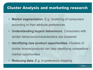


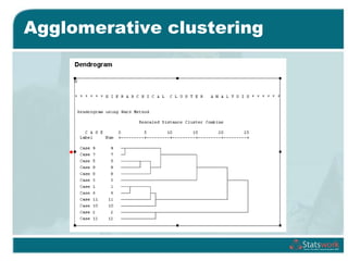


This document provides an overview of cluster analysis techniques used in marketing research. It defines cluster analysis as classifying cases into homogeneous groups based on a set of variables. Cluster analysis can be used for market segmentation, understanding buyer behaviors, and identifying new product opportunities in marketing research. The document outlines the steps to conduct cluster analysis, including selecting a distance measure and clustering algorithm, determining the number of clusters, and validating the analysis. It provides examples of hierarchical and non-hierarchical clustering methods like k-means and discusses choosing between these approaches. SPSS is used to demonstrate a cluster analysis example analyzing supermarket customer data.