Downloaded 25 times
![Optimal State Regulator
through the Matrix Riccati
Equation
Submitted to
Mrs. Shimi SL
Assistant Professor
Submitted By
Mr. Dhruv Upadhaya
162510
ME [ I&C ], Regular
4/17/2017 1Mr. Dhruv Upadhaya](https://image.slidesharecdn.com/ricatti-170417034312/75/Ricatti-Equation-1-2048.jpg)

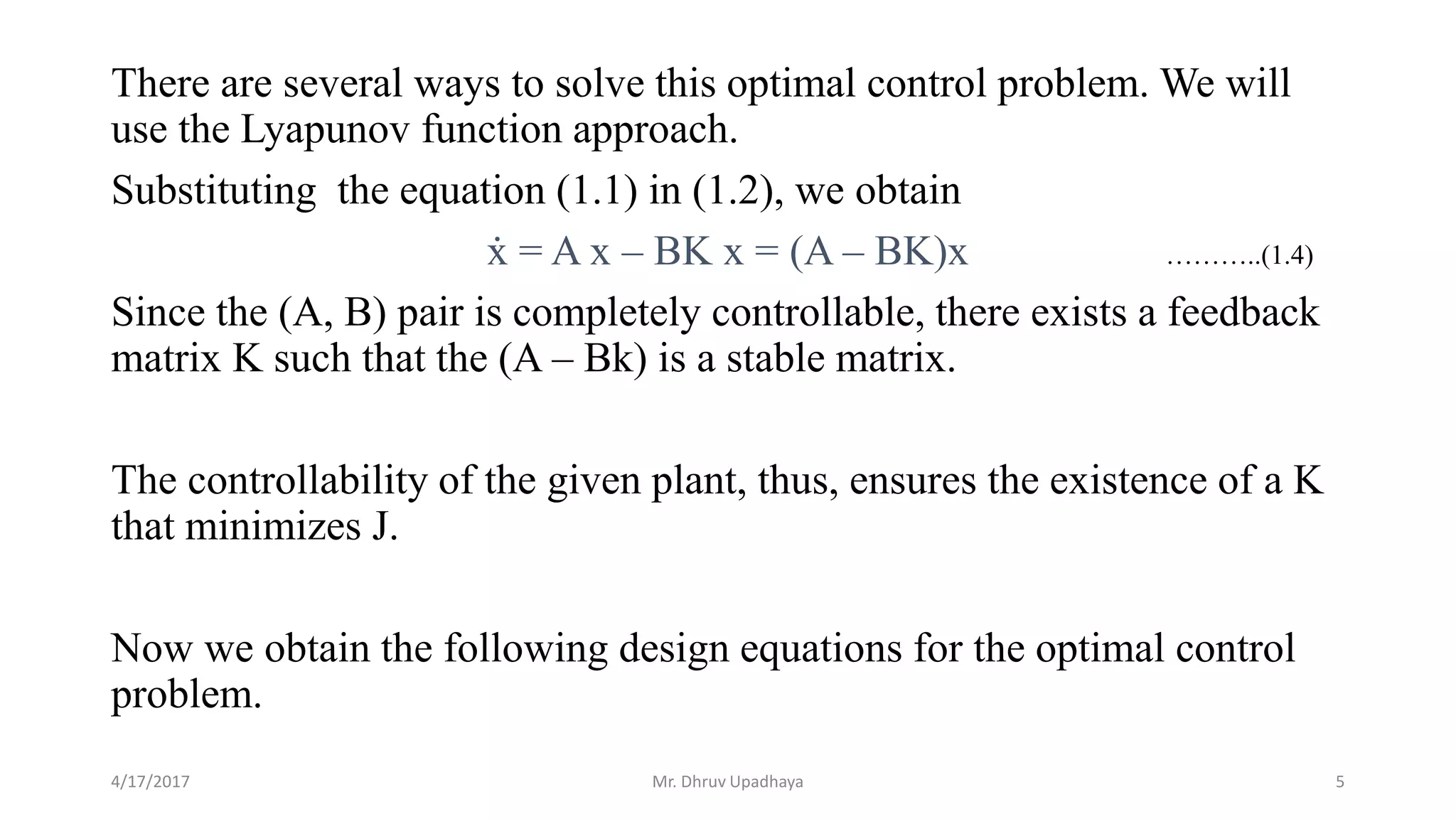


![ATP + PA – [ΓK – (ΓT)-1BTP]T [ΓK – (ΓT)-1BTP] – PBR-1BTP + Q= 0
The condition 1.9 for the unconstrained minimization of J leads to the
following equations :
𝜕
𝜕kij
[(ΓK – (ΓT)−1BTP)T (ΓK – (ΓT)−1BTP)] = 0
Since the matrix within brackets is non negative definite, the minimum
occurs when it is zero, or when
ΓK = (ΓT)−1BTP
Hence
K = Γ−1(ΓT)−1BTP = R−1BTP
4/17/2017 8
………..(1.10)
………..(1.11)
Mr. Dhruv Upadhaya](https://image.slidesharecdn.com/ricatti-170417034312/75/Ricatti-Equation-8-2048.jpg)


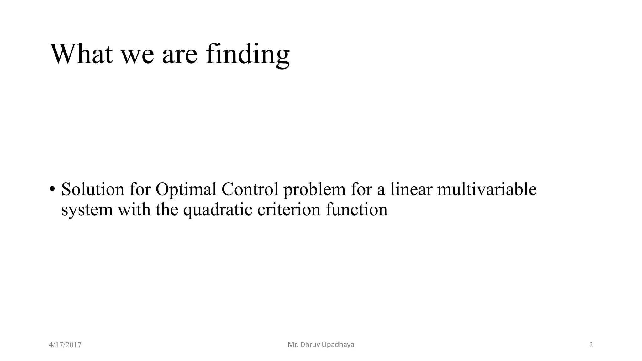
1. The document discusses solving the optimal control problem for a linear multivariable system using the matrix Riccati equation. 2. It describes the plant model and performance index, and derives the matrix Riccati equation and optimal control law. 3. Solving the matrix Riccati equation for a positive definite matrix P and substituting it into the optimal control law equation provides the solution to the optimal control problem.