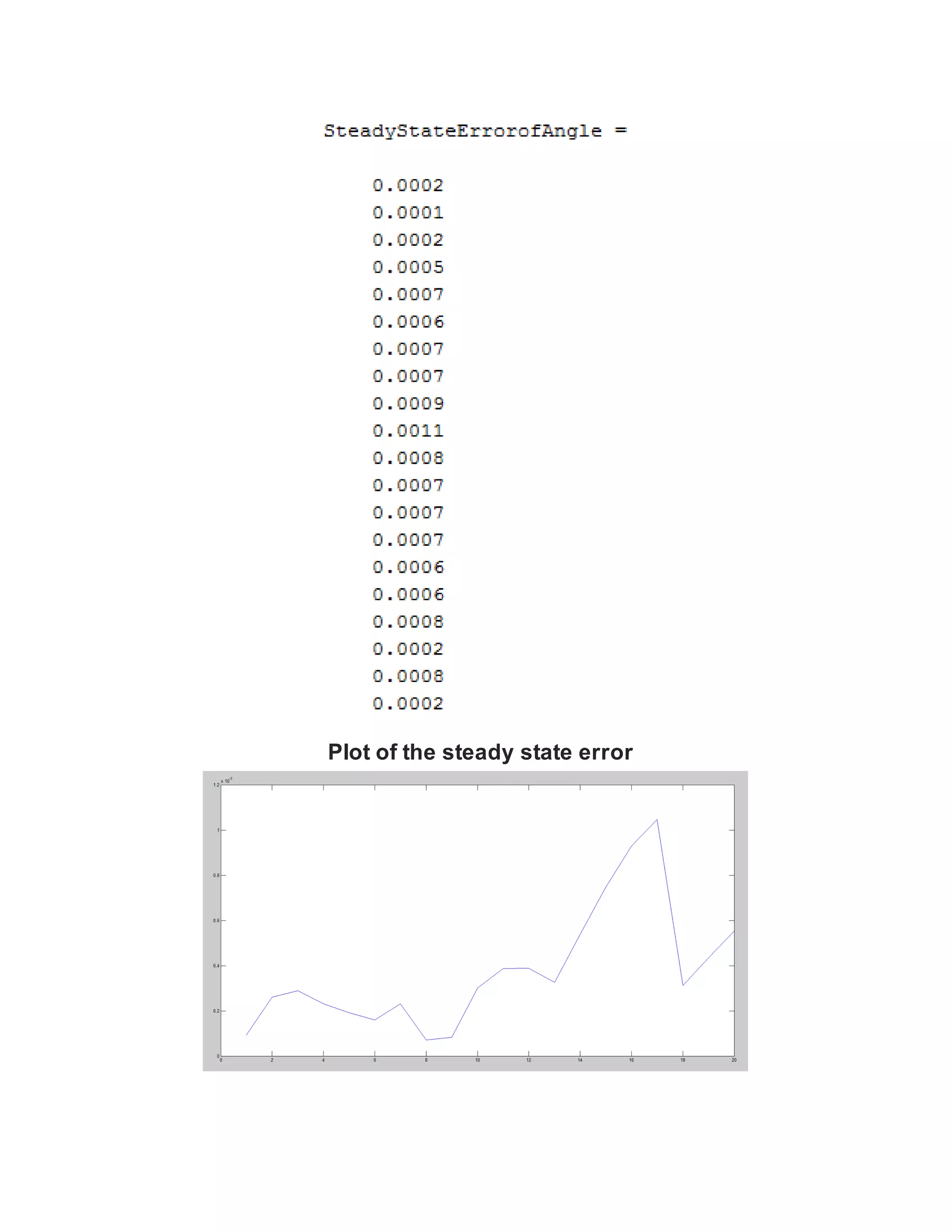
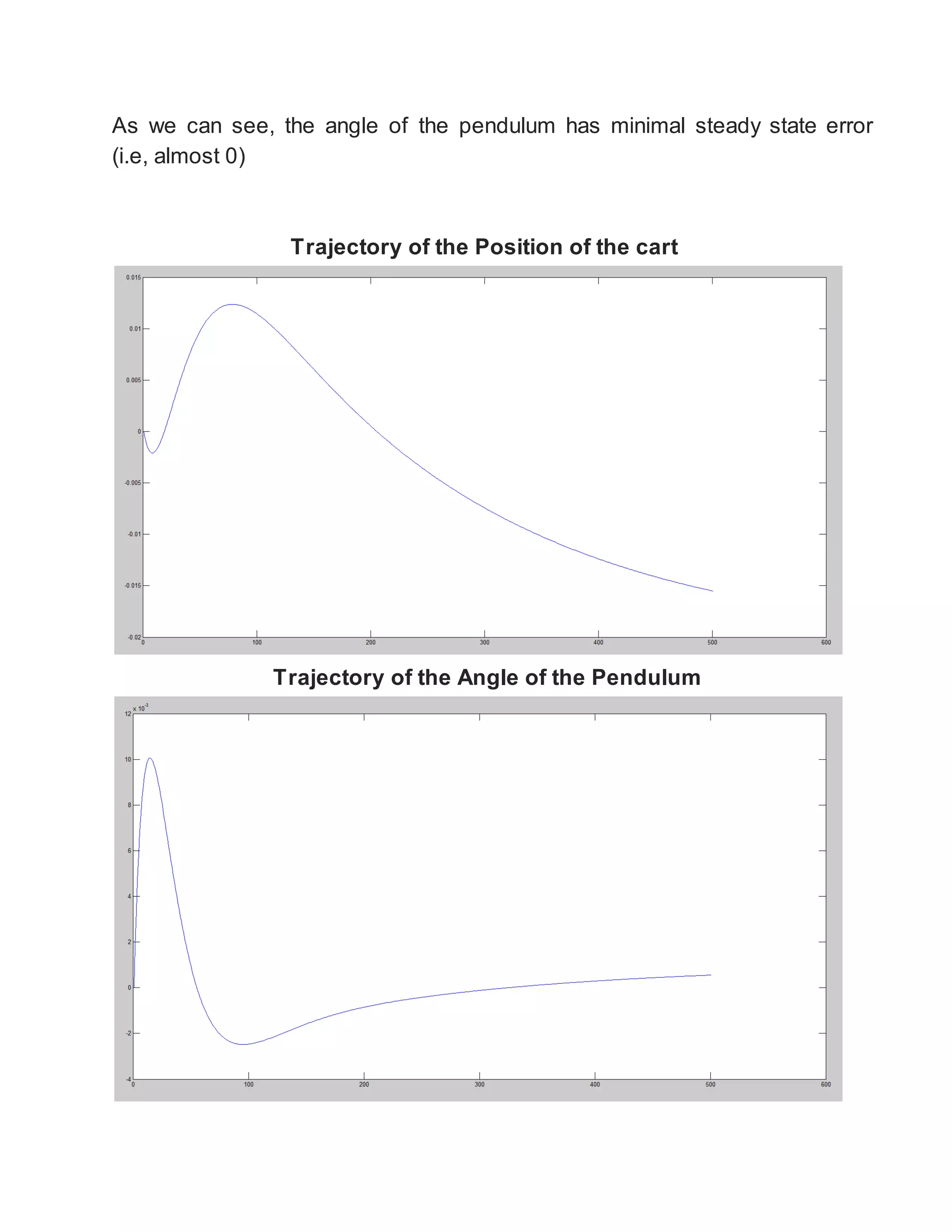
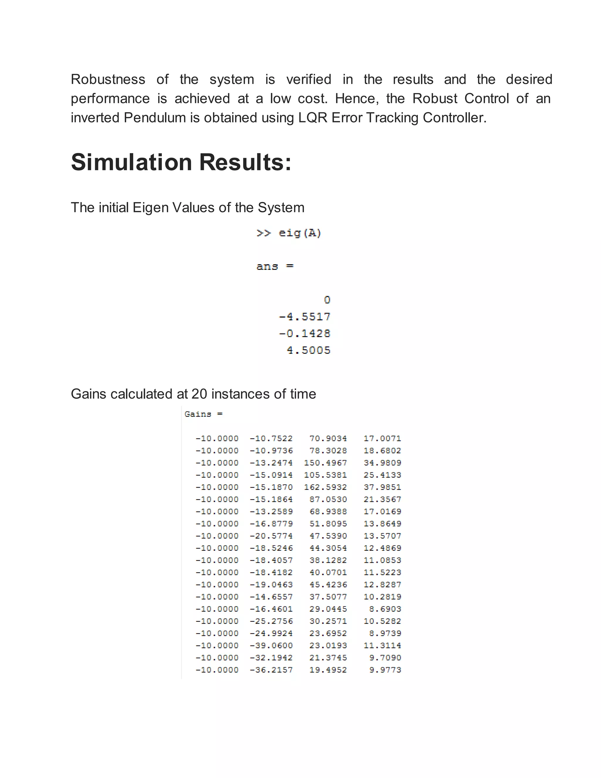
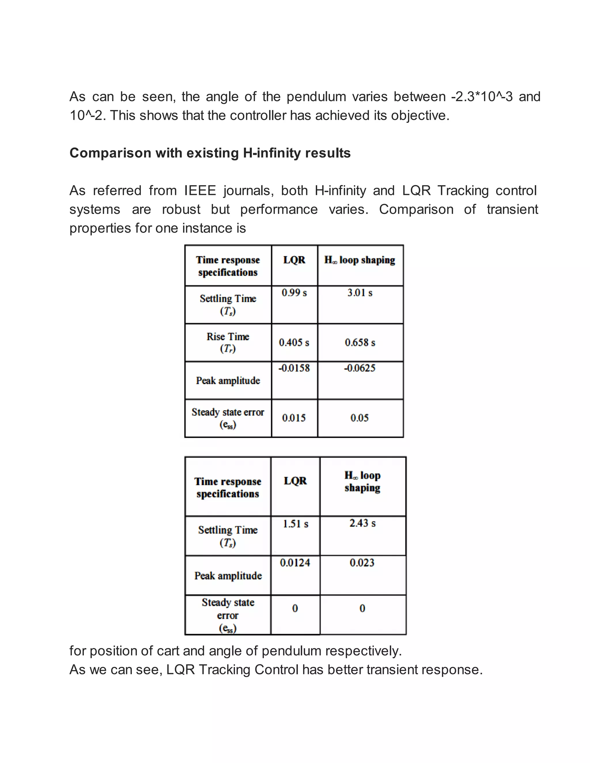
1) An LQR controller with feedforward control and steady state error tracking was designed and simulated to control an inverted pendulum system. 2) The LQR controller stabilized the unstable system and achieved good performance for the pendulum angle and cart position with minimal overshoot and steady state error. 3) Simulation results demonstrated the robustness of the designed controller under system uncertainties, showing improved performance over existing H-infinity control methods.

1. Robust Control of Inverted
Pendulum using LQR with
FeedForward control and Steady
State error tracking
EL7253: State Space Design for Linear Control Systems
by
Aniket Govindaraju
0507565
Department of Electrical and Computer Engineering
Polytechnic Institute of NYU
under
Dr. Prashanth Krishnamurthy
Department of Electrical and Computer Engineering

2. Abstract
The inverted pendulum is an unstable non-minimum phase plant, H-infinity
output feedback is far less robust. The objective is to determine the control
strategy that delivers better performance with respect to pendulum’s angle
and cart’s position. A Linear Quadratic Regulator with feedforward control
and steady state error tracking technique for controlling the linearized system
of the inverted pendulum model is presented. The result is compared against
previous H-infinity results obtained. Simulation study in MATLAB environment
shows that the LQR technique is capable of controlling the multi output
system successfully. A robust LQR Tracking controller is realized and results
show that good performance can be achieved and the uncertainities can be
compensated using the proposed controller.

3. Introduction
An Inverted Pendulum System is one of the most well known equipment in the
field of control systems theory. It is a non-linear problem which is linearized
in the control schemes. In general, the control of this system by classical
methods is a difficult task. This is mainly because the non-linear system has
two degrees of freedom (i.e, angle of the inverted pendulum and the position
of the cart) and only one control input.
The control strategies such as LQR and robust control is used to overcome
the Inverted Pendulum problem. Robust control scheme used in this paper is
a Linear Quadratic Regulator Tracking Controller with a FeedForward
controller. Performance of the pendulum’s angle and cart’s position is
assessed and presented.
Informally, a controller designed for a particular set of parameters is said to
be robust if it would also work well under a different set of assumptions.
High-gain feedback is a simple example of a robust control method; with
sufficiently high gain, the effect of any parameter variations will be negligible.
But high gains mean high control costs and performance costs. To avoid
that, a Linear Quadratic Controller is used.

4. System Modelling
The system in this example consists of an inverted pendulum mounted on a
motorized cart. The Inverted Pendulum system is unstable without control, i.e,
the cart needs to be controlled to balanced pendulum. Additionally the
dynamics of the system are non linear. The objective of the control system is
to balance the pendulum by applying force to the cart. A real world example
relates directly to this system is the attitude control of a booster rocket at
take-off.
In this case, we consider a two dimensional problem where the pendulum is
constrained to move in the vertical plane and the control input is the force F
that moves the cart horizontally and the outputs are the angle of the pendulum
and position of the cart.

5. For this example, let's assume the following quantities:
(M) mass of the cart 1 kg
(m) mass of the pendulum 0.4 kg
(b) coefficient of friction for cart 0.2 N/m/sec
(l) length to pendulum center of mass 0.6 m
(I) mass moment of inertia of the pendulum 0.012 kg.m^2
(F) force applied to the cart
(x) cart position coordinate
(theta) pendulum angle from vertical (down)
The dynamics of the system are given by

6. Summing the forces in the free-body diagram of the cart in the horizontal
direction, the following equation of motion is obtained
Summing the forces in the free-body diagram of the pendulum in the
horizontal direction, the following expression for the reaction force N is
obtained
Solving the two equations, we get
The sum of the forces perpendicular to the pendulum is,
To get rid of P and N, sum the moments about the centroid of the pendulum
to get the following equation,
Combining these last two expressions, you get the second governing
equation,
Let represent the deviation of the pendulum's position from equilibrium, that
is, = + . Again presuming a small deviation ( ) from equilibrium, we can
use the following small angle approximations of the nonlinear functions in our
system equations:

7. Hence, our governing equations become,
where F = u
Transfer Function
To obtain the transfer function of the linearized system equations, we take
laplace transform of the system equations,
And further solving the equations, we get
where
From the transfer function, we can cancel out the pole and zero at the origin
and that leads to,

8. State Space Model
By substituting the values in the model above, we get
System Performance
Using MATLAB, we can see that the poles of the system are at 0, -4.5517,
-0.1428 and 4.5005. As we can see, there is an unstable pole at 4.5005.
Impulse Response of Open loop system

9. As we can see from the plot, the system response is entirely unsatisfactory
and is unstable
Hence, we have to design a controller to stabilize the system and achieve
desirable performance of the system.
Controller Design
We use the LQR Tracking Controller to stabilize the system and also reduce
the control and performance cost. This controller also reduces the steady
state error of the system by employing a Steady State Error Tracking by
using a FeedForward loop to asymptotically tracking the error.
To use LQR, we first have to make sure the system is controllable and
observable. In this case, the Inverted Pendulum system satisfies that
condition.
The cost function is defined as

10. LQR minimizes the performance cost of the system using wieghting
parameters, Q and R for the states and input respectively. For this system,
we choose
R = 1 and Q = p*CT
C (where p is varied to obtain optimal cost)
In this case,
The (1,1) and (3,3) elements of the Q matrix provide weight to the state
variables corresponding to the position of the cart and angle of the pendulum
respectively. They can be increased for better performance but that would
increase the control cost. Hence, these values were selected to balance the
control cost and the performance cost.
The uncertainities of the system were treated as random disturbances to the
input u and sensor reading at the output y. To incorporate these
uncertainities in our design, randomly generated variable disturbances were
added to the system

11. The controller using LQR has the form
where P is found by solving the Algebraic Riccati Equation
and the optimal control law is given by
Now, the system obtained has good dynamic properties and has stabilized
using the optimal control law. But the steady state error has to be addressed.
Designing an Asymptotic Error Tracking
controller to reduce Steady State Error

12. where K is the LQR controller and the Error Tracking controller is
Now, the input u changes from -Kx to r - Kx, where is the
precompensator.
To find ,
The transfer system becomes,
And using K from the LQR, we have
The C matrix is modified to reflect the fact that the reference is a command
only on the cart position, i.e, only the first row of actual C matrix.

13. Designing an Observer
As we know, not all states can be accurately known at all times. Hence we
design an observer-based controller.
Now we can estimate our system state by the following equation,
The Complete System is now formed resulting in the following state space
equations,

14. Robustness of the system is verified in the results and the desired
performance is achieved at a low cost. Hence, the Robust Control of an
inverted Pendulum is obtained using LQR Error Tracking Controller.
Simulation Results:
The initial Eigen Values of the System
Gains calculated at 20 instances of time

15. As it can be seen, the gain matrix K adjusts its value at every instance to
maintain the desired system performance under uncertainity.
The Complete System State Space Model is given by,

16. And the eigen values of the final system are,
It can be seen that the system is stable as all the poles are in the left hand
side of the plane.
So far, we have seen that the design stabilized the system. Now we check its
performance and robustness.
All the graphs correspond to the system response with uncertainites (20
instances)

17. Impulse Response
As we can see from the graph, the settling time when the system is affected
by an Impulse is around 4 seconds for the angle of the pendulum (impulse
response of the second output) and the rise time and overshoot are also
minimal.
Step Response

18. Again, as observed in the plots, position(blue) has a small steady state error
(i.e, when the stystem reaches steady state, the position is at about 0.1) but
the angle(green) has negligible steady state error.
Bode Plot
From the above Bode Plot, the gain margin of the position and angle are
between 4 and 10 and the phase margin of both is infinite which indicates the
system is robust and has minimal overshoot. The problem with infinite phase
margin is that the system will have trouble tracking the signals. But this was
solved by adding the Steady State Error Tracking Controller. Hence, we have
a Robust Control System.
The Steady State error of the angle during the 20 instances

19. Plot of the steady state error

20. As we can see, the angle of the pendulum has minimal steady state error
(i.e, almost 0)
Trajectory of the Position of the cart
Trajectory of the Angle of the Pendulum

21. As can be seen, the angle of the pendulum varies between -2.3*10^-3 and
10^-2. This shows that the controller has achieved its objective.
Comparison with existing H-infinity results
As referred from IEEE journals, both H-infinity and LQR Tracking control
systems are robust but performance varies. Comparison of transient
properties for one instance is
for position of cart and angle of pendulum respectively.
As we can see, LQR Tracking Control has better transient response.

22. Conclusion
In this paper, an LQR Tracking Controller was successfully designed for te
Inverted Pendulum system. Based on the results, it is concluded that the
control method is capable of controlling the pendulum’s angle and cart’s
position of the linearized system. The controller has good transient
responses, optimized performance and control cost and is Robust. By
varying the values of the weight matrices, better performance can be
achieved at higher costs.
Since the Tracking controller was included in the design, the infinite phase
margin (which poses a tracking problem) is dealt with and the Steady State
error tracking improved the performance of the system. Since all the states
can not be observed, a full-order observer was also designed.
The resultant design was a Robust Control System for an Inverted Pendulum
System with desired performance and optimal cost.

23. References
1. Lee, S.S., and Lee, J.M, "Robust control of the inverted pendulum and mobile
robot," Assembly and Manufacturing, 2009. ISAM 2009. IEEE International
Symposium on , vol., no., pp.398-401, 17-20 Nov. 2009.
2. Zhang Jing, and Xu Lin, "Robust control of the inverted pendulum," Systems and
Control in Aerospace and Astronautics, 2008. ISSCAA 2008. 2nd International
Symposium on , vol., no., pp.1-3, 10-12 Dec. 2008.
3. Sek Un Cheang, and Wei Ji Chen, "Stabilizing control of an inverted pendulum
system based on a, loop shaping design procedure," Intelligent Control and
Automation, 2000. Proceedings of the 3rd World Congress on , vol.5, no.,
pp.3385-3388 vol.5, 2000.
4. J. Li and T.-C. Tsao, “Robust performance repetitive control systems,” ASME J.
Dynamic Systems, Measurement, and Control, vol. 123, no. 3, pp. 330-337, 2001.
5. T.-Y. Doh and M. J. Chung, “Repetitive control design for linear systems with
time-varying uncertainties,” IEE Proc. - Control Theory and Applications, vol. 150,
no. 4, pp. 427-432, 2003.
6. K. Zhou and J. C. Doyle, Essentials of Robust Control, Prentice-Hall, Inc., 1998.
7. M.-C. Tsai and W.-S. Yao, “Analysis and estimation of tracking errors of plug-in
type repetitive control system,” IEEE Trans. on Automatic Control, vol. 50, no. 8,
pp. 1190-1195, 2005.