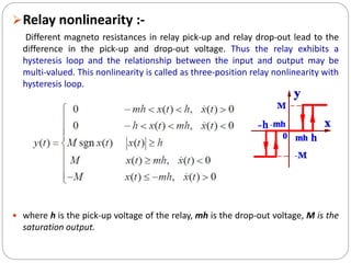
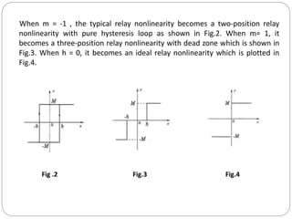
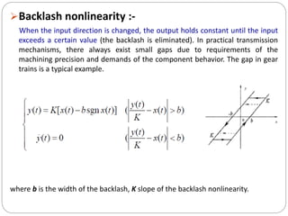
This document discusses nonlinear control systems using phase plane and phase trajectory methods. It defines nonlinear systems and common physical nonlinearities like saturation, dead zone, relay, and backlash. Phase plane analysis is introduced as a graphical method to study nonlinear systems using a plane with state variables x and dx/dt as coordinates. Key concepts are defined like phase plane, phase trajectory, and phase portrait. Methods for sketching phase trajectories include analytical solutions and graphical methods like isoclines. Examples are given to illustrate phase portraits for different linear systems.

1. Presented By:
NIRAJ SOLANKI
NONLINEAR CONTROL SYSTEM
(Phase plane & Phase Trajectory Method)

2.  What is Non-Linear System?
 Characteristics of Non-Linear System.
 Common physical Nonlinearities.
 Investigation of Non-Linear system by Different Methods.

3. Nonlinearities in Physics Systems
 Nonlinearity is the universal law.
 There are a lot of kinds of nonlinear systems and responses.
 The linear model is the approximate description of practical
systems under the specific conditions.
Typical Nonlinear Factors in Control Systems
SATURATION DEAD ZONE BACKLASH RELAY

4.  Saturation nonlinearity : -
The input and output exhibit a linear relationship in a certain range; when the
input exceeds this range, the output simply stays around its maximum value.
This nonlinearity is called saturation.
If x and y are the input and output signals of the nonlinear component and its
mathematical expression is:-
where α is the width of the linear zone, K the slope of the linear zone.
The saturation is usually caused by the limits of the component’s energy,
power, etc. Sometimes, the saturation is intentionally introduced to restrict
over loading.

5. Dead-zone nonlinearity:-
Many measurement components and actuators have dead zone. For example,
some actuators will not work if the input is small, and the output signal remains
zero until the input reaches a certain value. The nonlinearity that the output is
zero until the input exceeds a certain value is called as dead-zone nonlinearity.
where ∆ is the width of the dead zone, K the slope of the linear output.

6. Relay nonlinearity :-
Different magneto resistances in relay pick-up and relay drop-out lead to the
difference in the pick-up and drop-out voltage. Thus the relay exhibits a
hysteresis loop and the relationship between the input and output may be
multi-valued. This nonlinearity is called as three-position relay nonlinearity with
hysteresis loop.
 where h is the pick-up voltage of the relay, mh is the drop-out voltage, M is the
saturation output.

7. When m = -1 , the typical relay nonlinearity becomes a two-position relay
nonlinearity with pure hysteresis loop as shown in Fig.2. When m= 1, it
becomes a three-position relay nonlinearity with dead zone which is shown in
Fig.3. When h = 0, it becomes an ideal relay nonlinearity which is plotted in
Fig.4.
Fig .2 Fig.3 Fig.4

8. Backlash nonlinearity :-
When the input direction is changed, the output holds constant until the input
exceeds a certain value (the backlash is eliminated). In practical transmission
mechanisms, there always exist small gaps due to requirements of the
machining precision and demands of the component behavior. The gap in gear
trains is a typical example.
where b is the width of the backlash, K slope of the backlash nonlinearity.

9. Phase plane analysis is a graphical method for studying the first-
order and second-order linear or nonlinear systems.

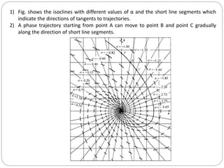
10.  Concepts of phase plane analysis
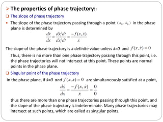
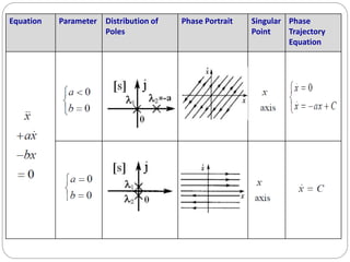
 Phase plane, phase trajectory and phase portrait :-
the second-order system by the following ordinary differential equation:
Where is the linear or non-linear function of x and
In respect to an input signal or with the zero initial condition .
The state space of this system is a plane having x and as coordinates which
is called as the phase plane.
 Thus one state of the system corresponds to each point in the plane x
As time t varies from zero to infinity,
change in state of the system in x-ẍ
plane is represented by the motion
of the point. The trajectory along
which the phase point moves is
called as phase trajectory. [shown in
fig 3(a) ]

11.  The properties of phase trajectory:-
 The slope of phase trajectory
 The slope of the phase trajectory passing through a point in the phase
plane is determined by
The slope of the phase trajectory is a definite value unless ẋ=0 and
Thus, there is no more than one phase trajectory passing through this point, i.e.
the phase trajectories will not intersect at this point. These points are normal
points in the phase plane.
 Singular point of the phase trajectory
In the phase plane, if ẋ=0 and are simultaneously satisfied at a point,
thus there are more than one phase trajectories passing through this point, and
the slope of the phase trajectory is indeterminate. Many phase trajectories may
intersect at such points, which are called as singular points.

12.  Direction of the phase trajectory:-
 In the upper half of the phase plane, ẋ >0 , the phase trajectory moves from
left to right along the x axis, thus the arrows on the phase trajectory point to
the right; similarly, in the lower half of the phase plane, ẋ <0 the arrows on the
phase trajectory point to the left. In a word, the phase trajectory moves
clockwise.
 Direction of the phase trajectory passing through the x axis.
 The phase trajectory always passes through x axis vertically. All points on the x
axis satisfy ẋ=0. thus except the singular point ƒ(x, ẋ)=0 , the slope of other
points is , indicating that the phase trajectory and x axis are
orthogonal.

13.  Sketching phase trajectories:-
 The sketching of the phase trajectory is the basis of phase plane analysis.
 Analytical method and graphical method are two main methods for
plotting the phase trajectory.
 The analytical method leads to a functional relationship between x and ẋ
by solving the differential equation, then the phase trajectory can be
constructed in the phase plane.
 The graphical method is used to construct the phase trajectory indirectly.

14.  Analytical method
 The analytical method can be applied when the differential equation is simple.
 consider a second-order linear system with non zero initial condition.

15. ………………………..(1)
Equ (1) represents the ellipse with the center
at the origin in the phase plane.
When the initial conditions are different, the
phase trajectories are a family of ellipses
starting from the point The phase
portrait is shown in Fig. indicting that the
response of the system is constant in
amplitude. The arrows in the figure indicate
the direction of increasing t . The phase portrait of the
undamped second-order system

16.  Graphical method:-
 There are a number of graphical methods, where method of isoclines is easy to
realize and widely used.
 The method of isoclines is a graphical method to sketch the phase trajectory.
From Equ.
the slope of the phase trajectory passing through a point is determined by
An isocline with slope of α can be defined as ………………(2)
 Equ.(2) is called as an isocline equation. the points on the isoclines all have the
same slope α
 By taking α to be different values, we can draw the corresponding isoclines in
the phase plane.
 The phase portrait can be obtained by sketching the continuous lines along the
field of directions

17.  Example 1:
Consider the system whose differential equation is ẍ+ẋ+x=0 ,sketch the phase
portrait of the system by using method of isoclines.
 Sol. :-
…………………………………(1)
Where, Equ.(1) is straight line equation with slope of
 We can obtain the corresponding slope of the isoclines with different values of
α.
 The slope of isoclines and the angle between the isoclines and x axis can be
found in table (1).

18. Table 1
Table 1, continued……….

19. 1) Fig. shows the isoclines with different values of α and the short line segments which
indicate the directions of tangents to trajectories.
2) A phase trajectory starting from point A can move to point B and point C gradually
along the direction of short line segments.

20.  The phase portrait of the second-order linear system
 The differential equation of the second-order linear system with zero input as
Thus,
………………………….(3)
 According to Equ.(3), the corresponding phase portrait can be obtained by the
method of isoclines or solving the phase trajectory equation
 The phase portraits of second-order linear systems under different situations
can be found in the Table (2).

21. Equation Parameter Distribution of
Poles
Phase Portrait Singular
Point
Phase
Trajectory
Equation

22. Equation Parameter Distribution of
Poles
Phase Portrait Singular
Point
Phase
Trajectory
Equation

23. Equation Parameter Distribution of
Poles
Phase Portrait Singular
Point
Phase
Trajectory
Equation
a is
arbitory,
b>0
(0,0)
Saddle
point
X-axis

24. Equation Parameter Distribution of
Poles
Phase Portrait Singular
Point
Phase
Trajectory
Equation