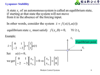
The document discusses various concepts related to stability analysis of control systems including:
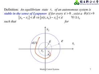
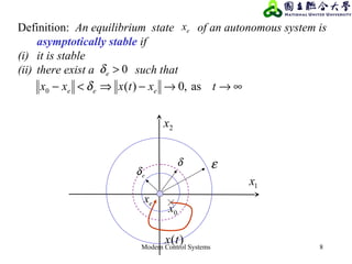
1) Bounded-input bounded-output (BIBO) stability, asymptotic stability, and Lyapunov stability.
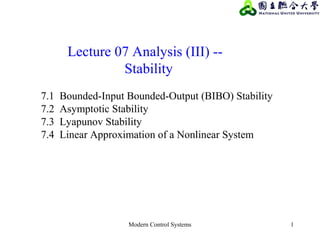
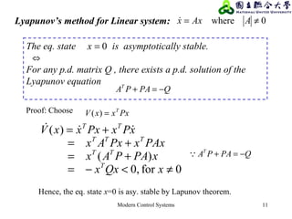
2) For linear systems, BIBO stability is equivalent to having all poles in the left half plane, while asymptotic stability requires all eigenvalues of the A matrix to have negative real parts.
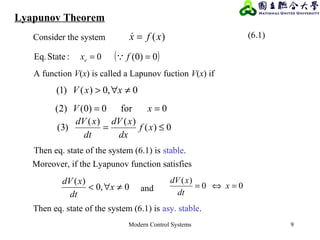
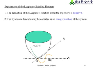
3) Lyapunov's stability theorem provides a method to analyze stability using a Lyapunov function that is positive definite and whose derivative is negative semi-definite.
![Modern Control Systems 3
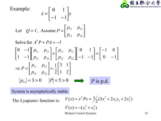
Asymptotically stable ⇔ All the eigenvalues of the A matrix
have negative real parts
(i.e. in the LHP)
∞→→
==
ttx
Axxtu
as0)(
systemthee.i.0,)(When
Cxy
BuAxx
=
+=
AsI
BAsIadjC
BAsIC
sq
sp
sT
−
−
=−== − ][
)(
)(
)(
)( 1
0=− AsI Solve for the eigenvalues for A matrix
Asymptotic stablility
Note: Asy. Stability is indepedent of B and C Matrix
For linear systems:](https://image.slidesharecdn.com/msclecture07-170411053937/85/Msc-lecture07-3-320.jpg)
![Modern Control Systems 4
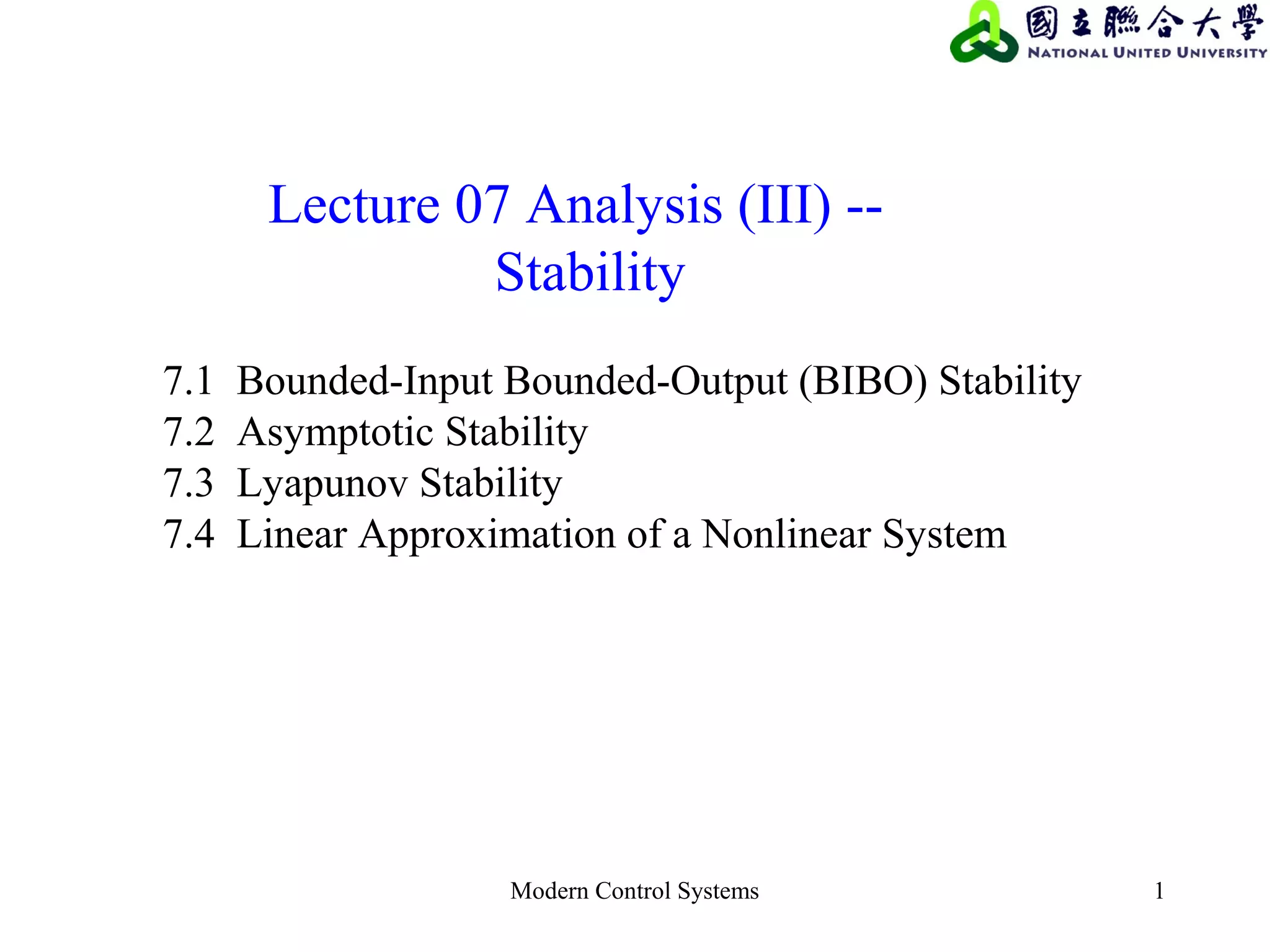
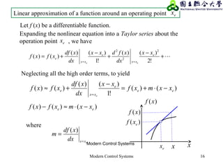
Asy. Stability from Model Decomposition
,n,ivAv iiii 1,satisfying,i.e. == λλ
Suppose that all the eigenvalues of A are distinct.
nn
RA ×
∈
CTC
BTB
ATTA
=
=
=
−
−
1
1
DuCTzy
BuTATzTz
+=
+= −− 11
ξξ ATT 1−
=
][ 21 n,v,, vvT =Coordinate Matrix
=
nnn
ξ
ξ
ξ
λ
λ
λ
ξ
ξ
ξ
2
1
2
1
2
1
00
0
000
000
Hence, system Asy. Stable ⇔ all the eigenvales of A at lie in the LHP
⇒
⇒
,)0()0()0()()( 2211
21
n
t
n
tt
ξevξevξevtTtx nλλλ
ζ +++== )0()0( 1
xTξ −
=
ivLet the eigenvector of matrix A with respect to eigenvalue iλ](https://image.slidesharecdn.com/msclecture07-170411053937/85/Msc-lecture07-4-320.jpg)
![Modern Control Systems 14
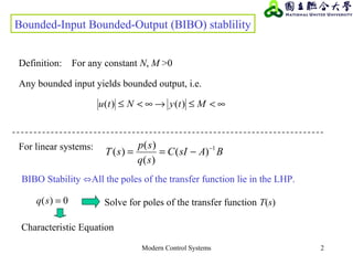
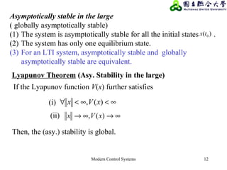
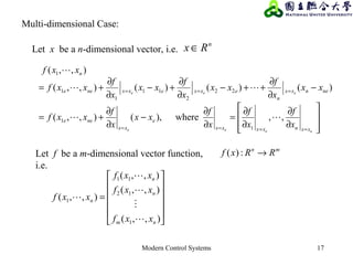
Remark:
(1) are all negative Q is n.d.
(2) All leading principle minors of –Q are positive Q is n.d.
nQQQ ,, 21
[ ]
[ ]
=
=
++++=
3
2
1
321
3
2
1
321
2
332
2
131
2
1
132
330
202
100
630
402
6342)(
x
x
x
xxx
x
x
x
xxx
xxxxxxxxV
024
06
02
3
2
1
<−=
>=
>=
Q
Q
Q
Q is not p.d.
Example:](https://image.slidesharecdn.com/msclecture07-170411053937/85/Msc-lecture07-14-320.jpg)
![Modern Control Systems 18
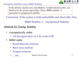
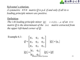
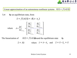
Special Case: n=m=2
)()()()( ee
xx
e xxAxx
x
f
xfxf
e
−=−
∂
∂
≈−
=
T
xxx ],[where 21= A
x
f
x
f
x
f
x
f
x
f
ee
ee
e
xxxx
xxxx
xx
=
∂
∂
∂
∂
∂
∂
∂
∂
=
∂
∂
==
==
=
2
2
1
2
2
1
1
1
and
Linear approximation of a function around an operating point ex](https://image.slidesharecdn.com/msclecture07-170411053937/85/Msc-lecture07-18-320.jpg)
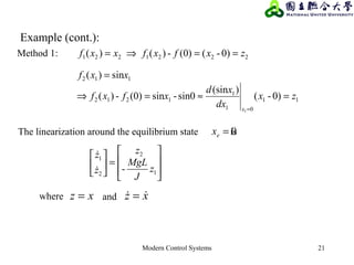
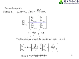
![Modern Control Systems 20
Example : Pendulum oscillator model
0sin2
2
=+ θ
θ
MgL
dt
d
J
From Newton’s Law we have
=
⇒
1
2
2
1
sin- x
J
MgL
x
x
x
θθ == 21 , xxDefine
We can show that is an equilibrium state.0=ex
where J is the inertia.
(Reproduced from [1])](https://image.slidesharecdn.com/msclecture07-170411053937/85/Msc-lecture07-20-320.jpg)


![Ph robust-and-optimal-control-kemin-zhou-john-c-doyle-keith-glover-603s[1]](https://cdn.slidesharecdn.com/ss_thumbnails/ph-robust-and-optimal-control-kemin-zhou-john-c-doyle-keith-glover-603s1-150521042530-lva1-app6891-thumbnail.jpg?width=640&height=640&fit=bounds)


