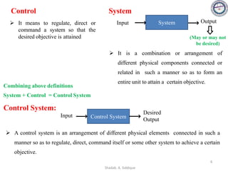
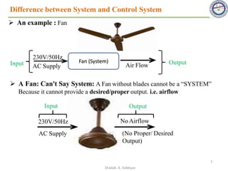
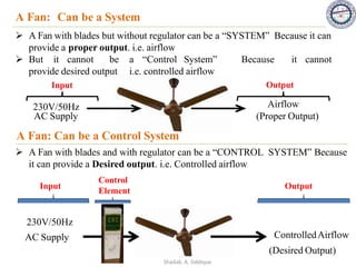
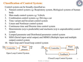
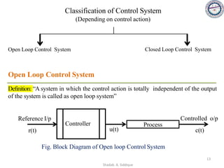
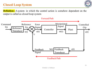
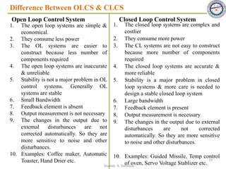
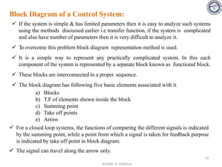
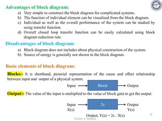
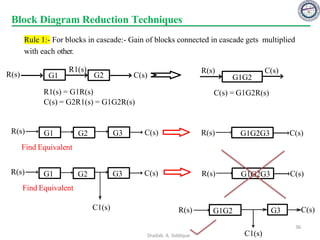
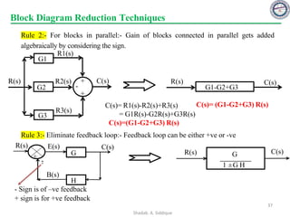
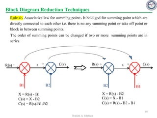
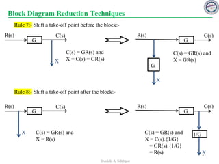
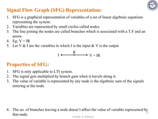
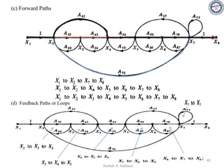
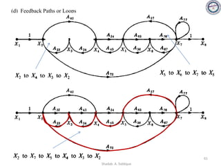
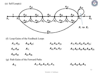
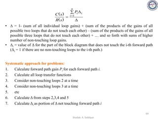
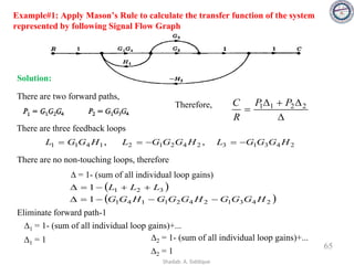
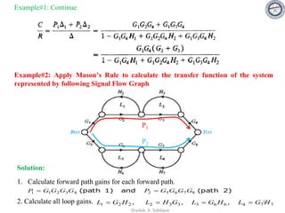
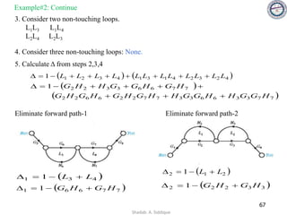
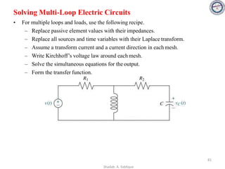
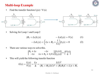
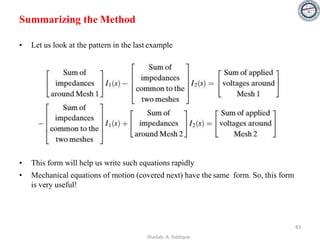
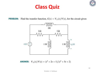
This document provides an overview of control systems including definitions, types, components, and their classifications such as open loop and closed loop systems. It also discusses the feedback mechanism, the role of various elements like controllers and plants, and the significance of modeling physical systems. The course aims to equip students with skills to analyze and differentiate between different control system responses and characteristics.


![Feedback and its Effect:
The effect of parameter variation on the system performance can be analyzed by
sensitivity of the system.
➢ Effect of Parameter variation in open loop control system:
Consider an open loop control system whose transfer function will be
G(s)
R(s) C(s) C(s)
R(s)
= G(s) = T(s)
C s = G s . R s
Let ∆G(s) be the changes in G(s) due to parameter variation, the corresponding
change in the output be ∆C(s)
C(s) + ∆C(s) = [G(s) + ∆G(s)] R(s)
= G(s) . R(s) + ∆G(s) . R(s)
C(s) + ∆C(s) = C(s) + ∆G(s) . R(s)
Therefore, ∆C(s) = ∆G(s) . R(s)
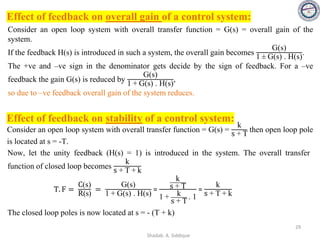
➢ Effect of Parameter variation in closed loop control system:
R(s)
G(s)
C(s)
H(s)
B(s)
+
±
E(s)
Consider a closed loop control system whose
transfer function is given by,
C(s) G(s)
=
R(s) 1 ± G(s).H(s)
TF = T(s) =
21
Shadab. A. Siddique](https://image.slidesharecdn.com/bec-26controlsystemsunit-ipdf-210419051634/85/BEC-26-control-Systems_unit-I_pdf-21-320.jpg)
![C(s) + ∆C(s)
R(s)
=
G(s) + ∆G(s)
1 ± [G(s) + ∆G(s)] . H(s)
C(s) + ∆C(s =
G(s) . R(s) + ∆G(s) . R(s)
1 ± [G(s) + ∆G(s)] . H(s)
∆C(s) =
G(s) . R(s) + ∆G(s) . R(s)
1 ± [G(s) + ∆G(s)] . H(s)
− C(s)
Assumption: G(s) . H(s) ≈ [G(s) + ∆G(s)] . H(s)
∆C(s) =
G(s) . R(s) + ∆G(s) . R(s)
1 ± G(s) . H(s)
− C(s)
∆C(s =
G(s) . R(s)
1 ± G(s) . H(s)
+
∆G(s) . R(s)
1 ± G(s) . H(s)
− C(s)
∆C(s = C s +
∆G(s) . R(s)
1 ± G(s) . H(s)
− C(s)
Therefore,
|1 ± G(s) . H(s)| ≥ 1
Let ∆G(s) be the changes in G(s) due to
parameter variation in system. The
corresponding change in the output is ∆C(s)
➢ Sensitivity of a control system:
An effect in the system parameters due to
parameter variation can be studied
mathematically by defining the term
sensitivity of a control system.
Let the variable in a system is varying by T
due to the variation in parameters K of the
system. The sensitivity of system
parameters K is expressed by,
S =
% Change in T
% Change in K
𝐾 𝑐𝑎𝑛 𝑏𝑒 𝑜𝑝𝑒𝑛 𝑙𝑜𝑜𝑝 𝑔𝑎𝑖𝑛 𝑜𝑟 𝑓𝑒𝑒𝑑𝑏𝑎𝑐𝑘
S =
d ln T
d ln K
=
∆T/T
∆K/K
=
𝝏T/T
𝝏K/K
𝑆𝐾
𝑇
=
K 𝝏T
𝑇 𝝏K
∆C(s) =
∆G(s) . R(s)
1 ± G(s) . H(s)
A symbolic representation 𝑆𝐾
𝑇
represents
the sensitivity of a variable T with respect
to the variation in the parameter K.
T may be the transfer function of output
variable & K may be the gain or feedback
factor.
22
Shadab. A. Siddique](https://image.slidesharecdn.com/bec-26controlsystemsunit-ipdf-210419051634/85/BEC-26-control-Systems_unit-I_pdf-22-320.jpg)
![SG
T
=
G(s) 𝜕𝑇
𝑇(𝑠) 𝜕𝐾
For open loop control system:
T(s) =
C(s)
R(s)
= G(s)
Forward path transfer function = Gain = G(s)
SG
T
=
G(s) 𝜕𝐺(𝑠)
𝐺(𝑠) 𝜕𝐺(𝑠)
= 1
---------------- (1)
SG
T
= 1
For closed loop control system:
T(s) =
C(s)
R(s)
= G(s) =
G(s)
1 + G(s) . H(s)
Forward path transfer function = Gain = G(s)
SG
T
=
G s
G(s)
1 + G(s) . H(s)
.
𝜕[
G(s)
1 + G(s) . H(s)
}
𝜕𝐺(𝑠)
SG
T
= [1 + G(s) . H(s)] .
1 + G(s)H(s) −G(s)H(s)
[1 + G(s)H(s)]2
SG
T
=
1
1 + G(s)H(s)
---------------- (2)
Comparing equation (1) and (2), it can be
observed that due to feedback the sensitivity
function get reduces by the factor
1
1 + G(s)H(s)
compared to an open loop
transfer function.
➢ Sensitivity of T(s) with H(s):
Let K be the gain ( forward path transfer function) & T be the overall transfer function of
the control system.
23
Shadab. A. Siddique Maj. G. S. Tripathi
Shadab. A. Siddique](https://image.slidesharecdn.com/bec-26controlsystemsunit-ipdf-210419051634/85/BEC-26-control-Systems_unit-I_pdf-23-320.jpg)
![➢ Sensitivity of T(s) with H(s):
Let us calculate the sensitivity function which indicates the sensitivity of overall transfer
function T(s) with respect to feedback path transfer function H(s). Such a function can be
expressed as,
SH
T
=
H(s) 𝜕𝑇(𝑠)
𝑇(𝑠) 𝜕𝐻(𝑠)
For closed loop control system,
T(s) =
C(s)
R(s)
= G(s) =
G(s)
1 + G(s)H(s)
Feedback path transfer function = H(s)
SH
T
=
H s
G(s)
1 + G(s)H(s)
.
𝜕[
G(s)
1 + G(s)H(s)
}
𝜕𝐻(𝑠)
SH
T
=
H(s) . [1 + G(s)H(s)]
G(s)
. [
−G(s)
[1 + G(s)H(s)]2 . G(s) ]
SH
T
=
− G(s)H(s)
1 + G(s)H(s)
---------------- (3)
It can be observed from equation (2) and (3) that the closed loop system is more sensitive
to variation in feedback path parameter than the variation in forward path parameter i.e.
gain. 24
Shadab. A. Siddique](https://image.slidesharecdn.com/bec-26controlsystemsunit-ipdf-210419051634/85/BEC-26-control-Systems_unit-I_pdf-24-320.jpg)
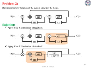
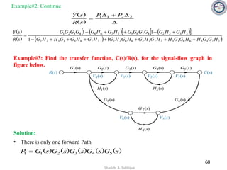
![Problem 2:
In the system shown in the figure, calculate the system sensitivity i SG1
T
(ii) SG2
T
and (ii) SH
T
R(s) C(s)
+
-
G1 G1
H
1
s + 1
1
s + 2
G1 = , G2 = and H = s
Solution:
[G1(s) . R(s) + H(s) . C(s)] . G2(s) = C(s)
G1 . R(s) . G2(s) = C(s) . [1 - H(s) . G2(s)]
T(s) =
C(s)
R(s)
=
G1(s) . G2(s)
1 + H(s) . G2(s)
(i) SG1
T
=
G1
T
.
𝜕T
𝜕G1
=
G1
G1G2
1 + G2H
𝜕
G1G2
1 + G2H
𝜕G1 =
1 + G2H
G2 .
G2 (1 + G2H)
(1 + HG2)2 = 1
(ii) SG2
T
=
G2
T
.
𝜕T
𝜕G2
=
G2
G1G2
1 + G2H
𝜕
G1G2
1 + G2H
𝜕G2 =
1 + G2H
G1 .
G1 (1 + G2H)− G1G2H
(1 + HG2)2 =
1
1 + G2H
(iii) SH
T
=
H
T
.
𝜕T
𝜕H
=
H
G1G2
1 + G2H
𝜕
G1G2
1 + G2H
𝜕H
=
H (1 + G2H)
G1G2
.
− G1 G2
(1 + HG2)2 . G2 =
− HG2
1 + G2H
SH
T
=
− HG2
1 + G2H
=
− s . 1
s + 2
1 + s . 1
s + 2
=
− s
2s + 2
SG2
T
=
1
1 + G2H
=
1
1 + s . 1
s + 2
=
s + 2
2s + 2
26
Shadab. A. Siddique](https://image.slidesharecdn.com/bec-26controlsystemsunit-ipdf-210419051634/85/BEC-26-control-Systems_unit-I_pdf-26-320.jpg)
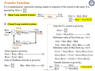
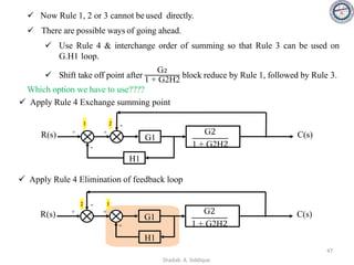
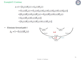
![E(s) = R(s) −B(s) and
C(s) =G.E(s) = G[R(s) − B(s)] =GR(s)−GB(s)
From Shown Figure,
But, B(s) =H.C(s)
C(s) =G.R(s)−G . H . C(s)
C(s) + G.H.C(s) = GR(s)
C(s)[1+G.H(s)]= G.R(s)
For Negative Feedback
C(s)
G
H
R(s)
−
B(s)
E(s)
For Positive Feedback
C(s)
G
H
R(s)
+
B(s)
E(s)
E(s) = R(s) +B(s) and
C(s) =G.E(s) = G[R(s) + B(s)] =GR(s)+GB(s)
From Shown Figure,
But, B(s) =H.C(s)
C(s) =G.R(s)+G . H . C(s)
C(s) −G.H.C(s) = GR(s)
C(s)[1−G.H(s)]= G.R(s)
+
+
C(s)
R(s)
=
G(𝑠)
1+G(s)H(s)
C(s)
R(s)
=
G(𝑠)
1− G(s)H(s)
Block Diagram Reduction Techniques
38
Shadab. A. Siddique](https://image.slidesharecdn.com/bec-26controlsystemsunit-ipdf-210419051634/85/BEC-26-control-Systems_unit-I_pdf-38-320.jpg)
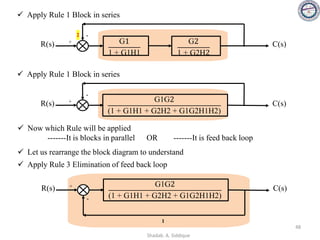
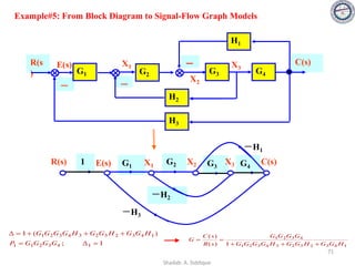
![Block Diagram Reduction Techniques
Rule 5:- Shift summing point before block:-
R(s) C(s)
X
+
G
C(s) = R(s)G + X C(s) = G [R(s) + X/G]
= GR(s) + X
+
C(s)
R(s) +
G
1/G
X
+
C(s)
R(s) +
G
X
C(s) = G [R(s)+X]
= GR(s)+GX
C(s) = GR(s)+XG
= GR(s)+XG
+
R(s) C(s)
X
+
G
G
+
Rule 6:- Shift summing point after block:-
40
Shadab. A. Siddique](https://image.slidesharecdn.com/bec-26controlsystemsunit-ipdf-210419051634/85/BEC-26-control-Systems_unit-I_pdf-40-320.jpg)
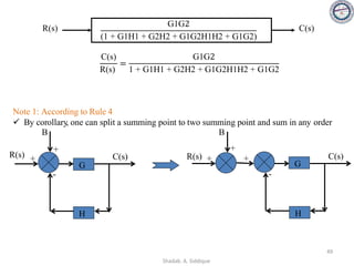
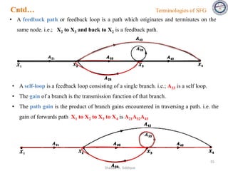
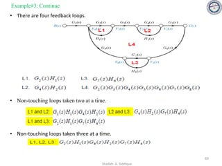
![58
Consider the signal flow graph below and identify the following
• Nontouching loop gains:
a) Input node: R(s)
b) Output node: C(s)
c) No of Forward paths: two
d) No. of Feedback paths (loops): four
e) Determine the loop gains of the feedback loops:
1. G2(s)H1(s)
2. G4(s)H2(s)
3. G4(s)G5(s)H3(s)
4. G4(s)G6(s)H3(s)
f) Determine the path gains of the forward paths:
1. G1(s) G2(s) G3(s) G4(s) G5(s) G7(s)
2. G1(s) G2(s) G3(s) G4(s) G6(s) G7(s)
g) Non-touching loops:
1. [G2(s)H1(s)][G4(s)H2(s)]
2. [G2(s)H1(s)][G4(s)G5(s)H3(s)]
3. [G2(s)H1(s)][G4(s)G6(s)H3(s)]
Shadab. A. Siddique](https://image.slidesharecdn.com/bec-26controlsystemsunit-ipdf-210419051634/85/BEC-26-control-Systems_unit-I_pdf-58-320.jpg)

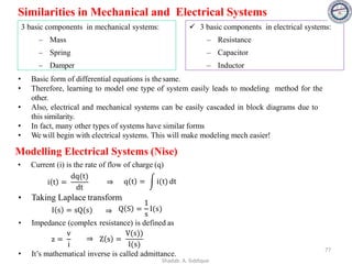
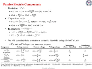
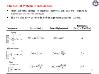
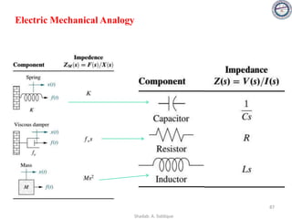
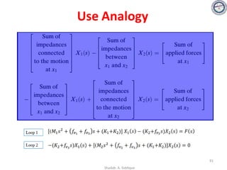
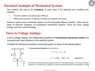
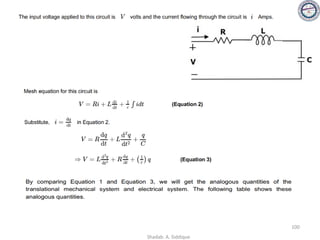
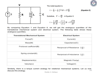
![Electrical/Mechanical Analogies
• Mechanical systems, like electrical networks, have 3 passive, linear components:
– Two of them (spring and mass) are energy-storage elements; one of them,
the viscous damper, dissipates energy.
– The two energy-storage elements are analogous to the two electrical
energy-storage elements, the inductor and capacitor. The energy dissipater
is analogous to electrical resistance.
• Displacement ‘x’ is analogous to current I
• Force ‘f’ is analogous to voltage ‘v’
• Impedance (Z=V/I) is therefore Z=F/X
• Since, [Sum of Impedances] I(s) = [Sum of applied voltages]
• Hence, [Sum of Impedances] X(s) = [Sum of applied forces]
86
Shadab. A. Siddique](https://image.slidesharecdn.com/bec-26controlsystemsunit-ipdf-210419051634/85/BEC-26-control-Systems_unit-I_pdf-86-320.jpg)