The document discusses variability and measures of variability. It defines variability as a quantitative measure of how spread out or clustered scores are in a distribution. The standard deviation is introduced as the most commonly used measure of variability, as it takes into account all scores in the distribution and provides the average distance of scores from the mean. Properties of the standard deviation are examined, such as how it does not change when a constant is added to all scores but does change when all scores are multiplied by a constant.

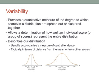
1. VARIABILITY
Behavioral Statistics
Summer 2017
Dr. Germano

2. Variability
• Provides a quantitative measure of the degree to which
scores in a distribution are spread out or clustered
together
• Allows a determination of how well an individual score (or
group of scores) represent the entire distribution
• Describes our distribution
• Usually accompanies a measure of central tendency
• Typically in terms of distance from the mean or from other scores

3. Which dataset
has more
variability?
0
2
4
6
8
10
12
0 1 2 3 4
Sample
Score

4. Variability Size Matters
• When variability is small
(Experiment A), it is easy to
see a difference between
distributions
• When variability is large
(Experiment B), differences
between distributions may
be obscured
Difference! ?

5. Which distribution has more variability?
The red one?
The green one?
The blue one?

6. Measures of Variability
• Variability can be measured with
• Range
• Standard deviation
• Variance
• Variability is determined by measuring distance
• The distance between score X1 and the mean of the distribution
• Remember central tendency
• Mean, Median, Mode
• There is no “right” or “wrong” measure of central tendency, but the
shape of the distribution will affect how you interpret these statistics
Related concepts

7. The Range
• The difference between the largest X value and the
smallest X value
range = Xmax - Xmin
If X = 2, 4, 6, 1, 8, 10
Then range = ?
(remember the real limits!)
range = 10.5 – 0.5 = 10
If we don’t account for real limits: range = 10 – 1 + 1
• When scores are whole numbers or discrete variables with numerical
scores, the range tells us the number of measurement categories
1, 2, 3, 4, 5, 6, 7, 8, 9, and 10

8. Is the range a
reliable measure
of variability?
Scores
40
23
19
23
22
21
18
19.5
20
23
21.5
18.5
17.5
16
0
5
10
15
20
25
30
35
40
45
0 1 2 3
Sample 1
(score x = 40 included)
range = 40.5 – 15.5 = 25
or
range = 40 – 16 + 1 = 25
Sample 2
(score x = 40 removed)
range = 23.5 - 15.5 = 8
or
range = 23 – 16 + 1 = 8
Scores (highlow)
40
23
23
23
22
21.5
21
20
19.5
19
18.5
18
17.5
16

9. The Standard Deviation (SD)
Standard = average
Deviation* = distance from the mean
• Approximates the average distance of scores from the
mean
• Provides the most information
• Takes into account all scores in the distribution
• Most commonly used measure of variability
*Deviation is calculated as: X - μ

10. SD: A Conceptual Walkthrough
X X – μ
(calc)
X - μ
2 (2 – 6) -4
4 (4 – 6) -2
6 (6 – 6) 0
8 (8 – 6) 2
10 (10 – 6) 4
ΣX – μ = 0
We are interested in the relationship
of each score to the mean. Thus,
sign (+/-) is important.
o A score of 4 is below the mean by 2
points (-2), and a score of 10 is above
the mean by 4 points (+4).
X = 2, 4, 6, 8, 10
N = 5 μ = 6
ΣX – μ = 0. Will this always be the case?
Yes. If the mean is the balance
point, the sum of scores above the
mean will be exactly equal to the
sum of scores below the mean.

11. SD: A Conceptual Walkthrough (cont’d)
X X – μ (X – μ)2
2 -4 16
4 -2 4
6 0 0
8 2 4
10 4 16
Σ(X – μ)2 = 40
If we square each individual deviation
score, we get rid of the sign (+/-)
• We now have a value we can take the
average of
X = 2, 4, 6, 8, 10
N = 5 μ = 6
40 ÷ 5 = 8 variance
Population variance: the mean of the
squared deviation scores
Remember that we are not interested
in squared distance.
• To convert back into our original measure
of distance:
Standard deviation: the square root
of variance
√8 = 2.83 SD

12. The Calculation
of Variance and
Standard
Deviation
Step 1 Step 2
Step 3
Step 4
Voila! Standard
Deviation!
Variance

13. SD: A Conceptual Walkthrough (cont’d)
X X – μ (X – μ)2
2 -4 16
4 -2 4
6 0 0
8 2 4
10 4 16
Σ(X – μ)2 = 40
SD provides the measure of average
distance of scores from the mean
• Given this set of scores, does this seem
reasonable?
• What if I obtained a standard deviation
value of 20?
X = 2, 4, 6, 8, 10
N = 5 μ = 6
SD = 2.83

14. Formulas for Calculating Variance and SD
• First a note on notation:
• You will use your calculator to check
your work
• DO NOT freak out
• All formulas will be given to you for exams
• This is a learning tool – so you “get” the
concepts of variance and SD
Sample
SD: s
Variance: s²
Population
SD: σ
Variance: σ²

15. Sum of Squares (SS)
• SS = the sum of squared deviation scores
• The definitional formula expresses SS in the conceptual
way explained previously:
•
• The computational formula provides the same answer, but
is easier to use when the mean is not a whole number
  2
)( XSS
N
X
XSS
2
2
)( 

16. A Demonstration of Both SS Methods
X X2 X – μ (X - μ)2
2 4 (2 – 6) = -4 16
4 16 (4 – 6) = -2 4
6 36 (6 – 6) = 0 0
8 64 (8 – 6) = 2 4
10 100 (10 – 6) = 4 16
ΣX = 30 ΣX2 = 220 Σ(X – μ) = 0 Σ(X – μ)2 = 40
Definitional
Formula
40180220
5
)30(
220
)( 22
2

 N
X
XSS
Computational
Formula

17. Variance and Standard Deviation
Sample
• Note that these explicitly show the definitional SS formula.
You can also solve using the computational SS formula.
Population
2
2
2
2
11
)(
.
11
)(
s
n
SS
n
MX
s
DeviationStd
n
SS
n
MX
s
Variance













Variance
s 2
=
(X -m)2
å
N
=
SS
N
Std.Deviation
s =
(X -m)2
å
N
=
SS
N
= s 2

18. Why are the formulas different?
Sample
• We want our sample statistic to be as representative of
the population parameter as possible.
• However, our samples will often be less variable than the
population
• We adjust for the biased estimate of sample variability by dividing
by n – 1 (degrees of freedom) instead of N
Population
Std.Deviation
s =
SS
n -1
Std.Deviation
s =
SS
N
Variance
s2
=
SS
n -1
Variance
s 2
=
SS
N

19. Degrees of Freedom (df)
Determine the number of scores in the sample
that are independent and free to vary
• If n = 3 and M = 5
• Then ΣX must equal what?
• M = ΣX ÷ n  5 = ΣX ÷ 3
• The first two scores have no restrictions
• They are independent values and could be any value
• The third score is restricted
• Can only be one value, based on the sum of the first
two scores (2 + 9 = 11)
• X3 MUST be 4
X
2
9
?
n = 3
M = 5
ΣX = 15
 3 × 5 = 15
 This score has no “freedom”
ΣX = ?

20. Understanding
SD Graphically
68.26%
94.46%
99.73%

21. Why is Knowing Variability Important?
Begin to think about how you might compare two
distributions, and how these factors might play a role in
your conclusions

22. Comprehension Check
If you have two samples:
• Sample 1: n = 25, M = 80
• Sample 2: n = 25, M = 80
Does a score of 85 mean the same thing?
• Consider if for sample 1: s = 1 and for sample 2: s = 10
• Which situation would a score of 85 be a “better” score?
• A score of 85 in sample one means that this score is 5 standard
deviations above the mean
• A score in sample two means that this score is ½ a standard
deviation above the mean

23. Comprehension
Check
Sample 1
n = 25, M = 80
s = 1
Sample 2
n = 25, M = 80
s = 10
80
In which situation would a score of 85 be a “better-
than-average” score?
Sample 178 79 81 82 8377
60 70 90 100 11050 Sample 2

24. Properties of the Standard Deviation
X
1
2
3
4
5
6
3.5
1.87
For X
n = 6
M = 3.5
SD = 1.87

25. Properties of the Standard Deviation
X
1
2
3
4
5
6
X + 1
2
3
4
5
6
7
3.5
1.87
4.5
1.87
For X
n = 6
M = 3.5
SD = 1.87
For X + 1
n = 6
M = 4.5
SD = 1.87

26. Properties of the Standard Deviation
X
1
2
3
4
5
6
X + 1
2
3
4
5
6
7
• Adding a constant to each score results in
the addition of the same constant to the M,
but no change in the SD (s or σ)
4.5
1.87
For X
n = 6
M = 3.5
SD = 1.87
For X + 1
n = 6
M = 4.5
SD = 1.87

27. Properties of the Standard Deviation
3.5
1.87
For X
n = 6
M = 3.5
SD = 1.87
X
1
2
3
4
5
6

28. Properties of the Standard Deviation
3.5
1.87
7
3.74
For X
n = 6
M = 3.5
SD = 1.87
For X × 2
n = 6
M = 7
SD = 3.74
X × 2
2
4
6
8
10
12
X
1
2
3
4
5
6

29. Properties of the Standard Deviation
• Multiplying every score by a constant results
in the multiplication by the same constant of
the M, and multiplication by the same
constant of the SD (s or σ)
7
3.74
For X
n = 6
M = 3.5
SD = 1.87
For X × 2
n = 6
M = 7
SD = 3.74
X × 2
2
4
6
8
10
12
X
1
2
3
4
5
6

30. Properties of
the Standard
Deviation
Why does the
standard deviation
change when we
multiply, but not when
we add?
0
1
2
3
4
5
6
0 2 4 6 8
Adding +1 to every score
Multiplying every score by 2
0
1
2
3
4
5
6
0 2 4 6 8 10 12 14
X X + 1 X × 2
1 2 2
2 3 4
3 4 6
4 5 8
5 6 10
6 7 12