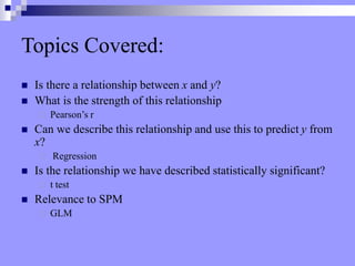
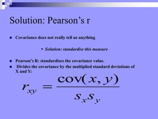
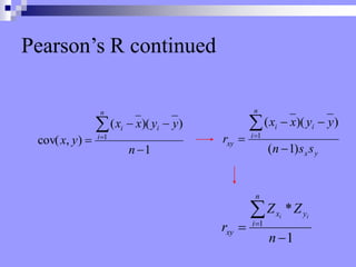
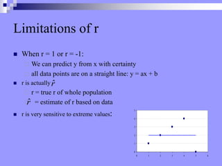
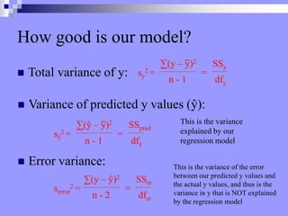
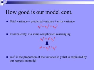
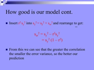
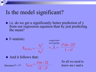
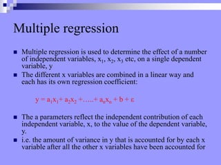
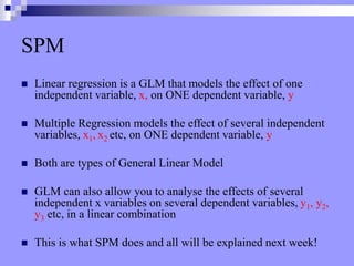
This document discusses correlation, regression, and the general linear model. It defines correlation as assessing the relationship between two variables, while regression describes how well one variable can predict another. Pearson's r standardizes the covariance between variables. Linear regression finds the best-fitting line that minimizes the residuals through the least squares method. The coefficient of determination, r-squared, indicates how much variance in the dependent variable is explained by the independent variable. Multiple regression extends this to include multiple independent variables. The general linear model encompasses both simple and multiple regression.

1. Correlation and
Regression
Davina Bristow &
Angela Quayle

2. Topics Covered:
 Is there a relationship between x and y?
 What is the strength of this relationship
 Pearson’s r
 Can we describe this relationship and use this to predict y from
x?
 Regression
 Is the relationship we have described statistically significant?
 t test
 Relevance to SPM
 GLM

3. The relationship between x and y
 Correlation: is there a relationship between 2
variables?
 Regression: how well a certain independent
variable predict dependent variable?
 CORRELATION  CAUSATION
In order to infer causality: manipulate independent
variable and observe effect on dependent variable

4. Scattergrams
Y
X
Y
X
Y
X
Y
Y Y
Positive correlation Negative correlation No correlation

5. Variance vs Covariance
 First, a note on your sample:
 If you’re wishing to assume that your sample is
representative of the general population (RANDOM
EFFECTS MODEL), use the degrees of freedom (n – 1)
in your calculations of variance or covariance.
 But if you’re simply wanting to assess your current
sample (FIXED EFFECTS MODEL), substitute n for
the degrees of freedom.

6. Variance vs Covariance
 Do two variables change together?
1
)
)(
(
)
,
cov( 1






n
y
y
x
x
y
x
i
n
i
i
Covariance:
• Gives information on the degree to
which two variables vary together.
• Note how similar the covariance is to
variance: the equation simply
multiplies x’s error scores by y’s error
scores as opposed to squaring x’s error
scores.
1
)
( 2
1
2





n
x
x
S
n
i
i
x
Variance:
• Gives information on variability of a
single variable.

7. Covariance
 When X and Y : cov (x,y) = pos.
 When X and Y : cov (x,y) = neg.
 When no constant relationship: cov (x,y) = 0
1
)
)(
(
)
,
cov( 1






n
y
y
x
x
y
x
i
n
i
i

8. Example Covariance
x y x
xi
 y
yi
 ( x
i
x  )( y
i
y  )
0 3 -3 0 0
2 2 -1 -1 1
3 4 0 1 0
4 0 1 -3 -3
6 6 3 3 9
3

x 3

y  7
75
.
1
4
7
1
))
)(
(
)
,
cov( 1








n
y
y
x
x
y
x
i
n
i
i What does this
number tell us?
0
1
2
3
4
5
6
7
0 1 2 3 4 5 6 7

9. Problem with Covariance:
 The value obtained by covariance is dependent on the size of
the data’s standard deviations: if large, the value will be
greater than if small… even if the relationship between x and y
is exactly the same in the large versus small standard
deviation datasets.

10. Example of how covariance value
relies on variance
High variance data Low variance data
Subject x y x error * y
error
x y X error * y
error
1 101 100 2500 54 53 9
2 81 80 900 53 52 4
3 61 60 100 52 51 1
4 51 50 0 51 50 0
5 41 40 100 50 49 1
6 21 20 900 49 48 4
7 1 0 2500 48 47 9
Mean 51 50 51 50
Sum of x error * y error : 7000 Sum of x error * y error : 28
Covariance: 1166.67 Covariance: 4.67

11. Solution: Pearson’s r
 Covariance does not really tell us anything
 Solution: standardise this measure
 Pearson’s R: standardises the covariance value.
 Divides the covariance by the multiplied standard deviations of
X and Y:
y
x
xy
s
s
y
x
r
)
,
cov(


12. Pearson’s R continued
1
)
)(
(
)
,
cov( 1






n
y
y
x
x
y
x
i
n
i
i
y
x
i
n
i
i
xy
s
s
n
y
y
x
x
r
)
1
(
)
)(
(
1






1
*
1




n
Z
Z
r
n
i
y
x
xy
i
i

13. Limitations of r
 When r = 1 or r = -1:
 We can predict y from x with certainty
 all data points are on a straight line: y = ax + b
 r is actually
 r = true r of whole population
 = estimate of r based on data
 r is very sensitive to extreme values:
0
1
2
3
4
5
0 1 2 3 4 5 6
r̂
r̂

14. Regression
 Correlation tells you if there is an association
between x and y but it doesn’t describe the
relationship or allow you to predict one
variable from the other.
 To do this we need REGRESSION!

15. Best-fit Line
= ŷ, predicted value
 Aim of linear regression is to fit a straight line, ŷ = ax + b, to data that
gives best prediction of y for any value of x
 This will be the line that
minimises distance between
data and fitted line, i.e.
the residuals
intercept
ε
ŷ = ax + b
ε = residual error
= y i , true value
slope

16. Least Squares Regression
 To find the best line we must minimise the sum of
the squares of the residuals (the vertical distances
from the data points to our line)
Residual (ε) = y - ŷ
Sum of squares of residuals = Σ (y – ŷ)2
Model line: ŷ = ax + b
 we must find values of a and b that minimise
Σ (y – ŷ)2
a = slope, b = intercept

17. Finding b
 First we find the value of b that gives the min
sum of squares
ε ε
b
b
b
 Trying different values of b is equivalent to
shifting the line up and down the scatter plot

18. Finding a
 Now we find the value of a that gives the min
sum of squares
b b b
 Trying out different values of a is equivalent to
changing the slope of the line, while b stays
constant

19. Minimising sums of squares
 Need to minimise Σ(y–ŷ)2
 ŷ = ax + b
 so need to minimise:
Σ(y - ax - b)2
 If we plot the sums of squares
for all different values of a and b
we get a parabola, because it is a
squared term
 So the min sum of squares is at
the bottom of the curve, where
the gradient is zero.
Values of a and b
sums
of
squares
(S)
Gradient = 0
min S

20. The maths bit
 The min sum of squares is at the bottom of the curve
where the gradient = 0
 So we can find a and b that give min sum of squares
by taking partial derivatives of Σ(y - ax - b)2 with
respect to a and b separately
 Then we solve these for 0 to give us the values of a
and b that give the min sum of squares

21. The solution
 Doing this gives the following equations for a and b:
a =
r sy
sx
r = correlation coefficient of x and y
sy = standard deviation of y
sx = standard deviation of x
 From you can see that:
 A low correlation coefficient gives a flatter slope (small value of
a)
 Large spread of y, i.e. high standard deviation, results in a
steeper slope (high value of a)
 Large spread of x, i.e. high standard deviation, results in a flatter
slope (high value of a)

22. The solution cont.
 Our model equation is ŷ = ax + b
 This line must pass through the mean so:
y = ax + b b = y – ax
 We can put our equation for a into this giving:
b = y – ax
b = y -
r sy
sx
r = correlation coefficient of x and y
sy = standard deviation of y
sx = standard deviation of x
x
 The smaller the correlation, the closer the
intercept is to the mean of y

23. Back to the model
 If the correlation is zero, we will simply predict the mean of y for every
value of x, and our regression line is just a flat straight line crossing the
x-axis at y
 But this isn’t very useful.
 We can calculate the regression line for any data, but the important
question is how well does this line fit the data, or how good is it at
predicting y from x
ŷ = ax + b =
r sy
sx
r sy
sx
x + y - x
r sy
sx
ŷ = (x – x) + y
Rearranges to:
a b
a a

24. How good is our model?
 Total variance of y: sy
2 =
∑(y – y)2
n - 1
SSy
dfy
=
 Variance of predicted y values (ŷ):
 Error variance:
sŷ
2 =
∑(ŷ – y)2
n - 1
SSpred
dfŷ
=
This is the variance
explained by our
regression model
serror
2 =
∑(y – ŷ)2
n - 2
SSer
dfer
=
This is the variance of the error
between our predicted y values and
the actual y values, and thus is the
variance in y that is NOT explained
by the regression model

25.  Total variance = predicted variance + error variance
sy
2 = sŷ
2 + ser
2
 Conveniently, via some complicated rearranging
sŷ
2 = r2 sy
2
r2 = sŷ
2 / sy
2
 so r2 is the proportion of the variance in y that is explained by
our regression model
How good is our model cont.

26. How good is our model cont.
 Insert r2 sy
2 into sy
2 = sŷ
2 + ser
2 and rearrange to get:
ser
2 = sy
2 – r2sy
2
= sy
2 (1 – r2)
 From this we can see that the greater the correlation
the smaller the error variance, so the better our
prediction

27. Is the model significant?
 i.e. do we get a significantly better prediction of y
from our regression equation than by just predicting
the mean?
 F-statistic:
F(dfŷ,dfer) =
sŷ
2
ser
2
=......=
r2 (n - 2)2
1 – r2
complicated
rearranging
 And it follows that:
t(n-2) =
r (n - 2)
√1 – r2
(because F = t2)
So all we need to
know are r and n

28. General Linear Model
 Linear regression is actually a form of the
General Linear Model where the parameters
are a, the slope of the line, and b, the intercept.
y = ax + b +ε
 A General Linear Model is just any model that
describes the data in terms of a straight line

29. Multiple regression
 Multiple regression is used to determine the effect of a number
of independent variables, x1, x2, x3 etc, on a single dependent
variable, y
 The different x variables are combined in a linear way and
each has its own regression coefficient:
y = a1x1+ a2x2 +…..+ anxn + b + ε
 The a parameters reflect the independent contribution of each
independent variable, x, to the value of the dependent variable,
y.
 i.e. the amount of variance in y that is accounted for by each x
variable after all the other x variables have been accounted for

30. SPM
 Linear regression is a GLM that models the effect of one
independent variable, x, on ONE dependent variable, y
 Multiple Regression models the effect of several independent
variables, x1, x2 etc, on ONE dependent variable, y
 Both are types of General Linear Model
 GLM can also allow you to analyse the effects of several
independent x variables on several dependent variables, y1, y2,
y3 etc, in a linear combination
 This is what SPM does and all will be explained next week!