Downloaded 92 times

![OXFORD
UNIVERSITY PRESS
Great Clarendon Street, Oxford OX2 6DP
Oxford University Press is a department of the University of Oxford.
It furthers the University's objective of excellence in research, scholarship,
and education by publishing worldwide in
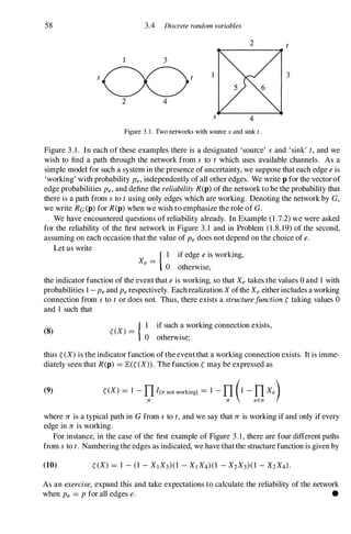
Oxford New York
Athens Auckland Bangkok Bogota Buenos Aires Cape Town
Chennai Dar es Salaam Delhi Florence Hong Kong Istanbul Karachi
Kolkata Kuala Lumpur Madrid Melbourne Mexico City Mumbai Nairobi
Paris Sao Paulo Shanghai Singapore Taipei Tokyo Toronto Warsaw
with associated companies in Berlin Ibadan
Oxford is a registered trade mark of Oxford University Press
in the UK and in certain other countries
Published in the United States
by Oxford University Press Inc., New York
© Geoffrey R. Grimmett and David R. Stirzaker 1982, 1992, 2001
The moral rights of the author have been asserted
Database right Oxford University Press (maker)
First edition 1982
Second edition 1992
Third edition 2001
All rights reserved. No part of this publication may be reproduced,
stored in a retrieval system, or transmitted, in any form or by any means,
without the prior permission in writing of Oxford University Press,
or as expressly permitted by law, or under terms agreed with the appropriate
reprographics rights organization. Enquiries concerning reproduction
outside the scope of the above should be sent to the Rights Department,
Oxford University Press, at the address above
You must not circulate this book in any other binding or cover
and you must impose this same condition on any acquirer
A catalogue record for this title is available from the British Library
Library of Congress Cataloging in Publication Data
Data available
ISBN 0 19 857223 9 [hardback]
ISBN 0 19 857222 0 [paperback]
10 9 8 7 6 5 4 3 2 1
Typeset by the authors
Printed in Great Britain
on acid-free paper by BiddIes Ltd, Guildford & King's Lynn](https://image.slidesharecdn.com/grimmettstirzaker-probabilityandrandomprocessesthirded2001-220507085451-bb31ac14/85/Grimmett-Stirzaker-Probability-and-Random-Processes-Third-Ed-2001-pdf-3-320.jpg)

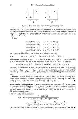
![1 .3 Probability 5
ratio is 1 . Furthermore, suppose that A and B are two disjoint events, each of which may or
may not occur at each trial. Then
N(AU B) = N(A) + N(B)
and so the ratio N(AU B)/N is the sum of the two ratios N(A)/N and N(B)/N. We now
think of these ratios as representing the probabilities of the appropriate events. The above
relations become
IP'(AU B) = IP'(A) + IP'(B), 1P'(0) = 0, IP'(Q) = 1 .
This discussion suggests that the probability function IP' should befinitely additive, which is
to say that
a glance at Example (1 .2.4) suggests the more extensive property that IP'be countablyadditive,
in thatthe correspondingproperty should hold forcountable collections AI, A2, . . . ofdisjoint
events.
These relations are sufficient to specify the desirable properties of a probability function IP'
applied to the set of events. Any such assignment oflikelihoods to the members of F is called
aprobability measure. Some individuals refer informally to IP' as a 'probability distribution',
especially when the sample space is finite or countably infinite; this practice is best avoided
since the term 'probability distribution' is reserved for another purpose to be encountered in
Chapter 2.
(1) Definition. A probability measure.lP' on (0, F) is a function.lP' : :F -+ [0, 1] satisfying
(a) .IP'(0) = 0, .IP'(O) = 1;
(b) if AI, Az, . • . is a collection ofdisjoint members of:F, in that Ai n Aj = 0 for all pairs
i. j satisfying i ::j:. j, then
The triple (Q, F,.IP'), comprising a set 0, a a-field F of subsets of 0, and a probability
measure .IP' on (0, F), is called a probability space.
A probability measure is a special example of what is called a measure on the pair (Q, F).
A measure is a function f.L : F -+ [0, 00) satisfying f.L(0) = 0 together with (b) above. A
measure f.Lis a probability measure if f.L(Q) = 1 .
We can associate a probability space (Q, F , IP') with any experiment, and all questions
associated with the experiment can be reformulated in terms of this space. It may seem
natural to ask for the numerical value of the probability IP'(A) of some event A. The answer
to such a question must be contained in the description of the experiment in question. For
example, the assertion that a/air coin is tossed once is equivalent to saying that heads and
tails have an equal probability of occurring; actually, this is the definition of fairness.](https://image.slidesharecdn.com/grimmettstirzaker-probabilityandrandomprocessesthirded2001-220507085451-bb31ac14/85/Grimmett-Stirzaker-Probability-and-Random-Processes-Third-Ed-2001-pdf-16-320.jpg)
![6 1 .3 Events and their probabilities
(2) Example. A coin, possibly biased, is tossed once. We can takeQ = {H, T} and :F =
{0, H, T,Q}, and a possible probability measure JP' : :F � [0, 1] is given by
JP'(0) = 0, JP'(H) = p, JP'(T) = 1 - p, JP'(Q) = 1 ,
where p is a fixed real number in the interval [0, 1 ] . If p = 1, then we say that the coin is
fair, or unbiased. •
(3) Example. A die is thrown once. We can takeQ = { l , 2, 3, 4, 5, 6}, :F ={O, l }n, and
the probability measure JP' given by
JP'(A) = LPi for any A S;Q,
iEA
where PI, P2, . . . , P6 are specified numbers from the interval [0, 1] having unit sum. The
probability that i turns up is Pi. The die is fair if Pi = i for each i, in which case
JP'(A) = ilAI for any A S;Q,
where IAI denotes the cardinality of A. •
The triple (Q, :F, JP') denotes a typical probability space. We now give some of its simple
but important properties.
(4) Lemma.
(a) JP'(AC) = 1 - JP'(A),
(b) ifB ;2 A then JP'(B) = JP'(A) + JP'(B A) 2: JP'(A),
(c) JP'(AU B) = JP'(A) + JP'(B) - JP'(A n B),
(d) more generally, ifAI, A2, . . . , An are events, then
II' (�A;) � �II'(A;) - t111'(A; n Aj) + ;f.II'(A; n Aj n A.) - . . .
+ (_I)n+IJP'(AI n A2 n . . . n An)
where,for example, Li<j sums over all unorderedpairs (i, j) with i =1= j.
Proof.
(a) AU AC = Q and A n AC = 0, so JP'(AU AC) = JP'(A) + JP'(N) = 1 .
(b) B = AU (B A). This is the union of disjoint sets and therefore
JP'(B) = JP'(A) + JP'(B A).
(c) AU B = AU (B A), which is a disjoint union. Therefore, by (b),
JP'(AU B) = JP'(A) + JP'(B A) = JP'(A) + JP'(B (A n B»
= JP'(A) + JP'(B) - JP'(A n B).
(d) The proof is by induction on n, and is left as an exercise (see Exercise (1.3.4» . •](https://image.slidesharecdn.com/grimmettstirzaker-probabilityandrandomprocessesthirded2001-220507085451-bb31ac14/85/Grimmett-Stirzaker-Probability-and-Random-Processes-Third-Ed-2001-pdf-17-320.jpg)
![1 .3 Probability 7
In Lemma (4b), B A denotes the set of members of B which are not in A. In order to
write down the quantity lP'(B A), we require that B A belongs to F, the domain oflP'; this is
always true when A and B belong to F, andto prove this was part ofExercise (1 .2.2). Notice
thateach proofproceeded by expressing an event in terms ofdisjoint unions and then applying
lP'. It is sometimes easier to calculate the probabilities of intersections of events rather than
their unions; part (d) ofthe lemma is useful then, as we shall discover soon. The next property
oflP' is more technical, and says that lP' is a continuous set function; this property is essentially
equivalent to the condition that lP' is countably additive rather than just finitely additive (see
Problem (1 .8. 16) also).
(5) Lemma. Let A I , A2, . . . be an increasing sequence ofevents, so that Al S; A2 S; A3 S;
. . " and write Afor their limit:
Then lP'(A) =limi--->oo lP'(Ai).
00
A =U Ai =.lim Ai .
1--->00
i=1
Similarly, ifBI , B2, . . . is a decreasing sequence ofevents, so that BI ;::> B2 ;::> B3 ;::> . • "
then
satisfies lP'(B) =limi--->oo lP'(Bi).
00
B =n Bi =.lim Bi
1--->00
i=1
Proof. A =AI U (A2 A I )U (A3 A2)U . .
. is the union of a disjoint family of events.
Thus, by Definition (1),
00
lP'(A) =lP'(AI) + LlP'(Ai+1 Ai)
i=1
n-I
=lP'(A I) + lim "' [lP'(Ai+l ) - lP'(Ai)]
n---7-oo L.....
i=1
To show the result for decreasing families of events, take complements and use the first part
(exercise). •
To recapitulate, statements concerning chance are implicitly related to experiments or
trials, the outcomes of which are not entirely predictable. With any such experiment we can
associate a probability space (Q, F, lP') the properties of which are consistent with our shared
and reasonable conceptions of the notion of chance.
Here is some final jargon. An event A is called null if lP'(A) =O. If lP'(A) =1, we say
that A occurs almost surely. Null events should not be confused with the impossible event
0. Null events are happening all around us, even though they have zero probability; after all,
what is the chance that a dart strikes any given point of the target at which it is thrown? That
is, the impossible event is null, but null events need not be impossible.](https://image.slidesharecdn.com/grimmettstirzaker-probabilityandrandomprocessesthirded2001-220507085451-bb31ac14/85/Grimmett-Stirzaker-Probability-and-Random-Processes-Third-Ed-2001-pdf-18-320.jpg)
![10 1 .4 Events and theirprobabilities
The usual dangerous argument contains the assertion
lP'(BB l one child is a boy) =lP'(other child is a boy).
Why is this meaningless? [Hint: Consider the sample space.] •
The next lemma is crucially important in probability theory. A family Bl, B2, . . . , Bn of
events is called a partition of the set Q if
n
Bi n Bj = 0 when i =I- j, and U Bi =Q.
i=1
Each elementary event (J) E Q belongs to exactly one set in a partition of Q.
(4) Lemma. Forany events A and B such that 0 < lP'(B) < 1,
lP'(A) = p(Ai I B)P(B) + lP'(A I BC)lP'(BC).
More generally. let B1. B2•• • . , Bn be a partition off'!. such that lP'(B/) > Ofor all i. Then
n
lP'(A) = LlP'(A I B;)lP'(Bj).
i=1
Proof. A =(A n B)U (A n BC). This is a disjoint union and so
lP'(A) =lP'(A n B) + lP'(A n BC)
=lP'(A I B)lP'(B) + lP'(A I BC)lP'(BC).
The second part is similar (see Problem (1 .8. 10» . •
(5) Example. We are given two urns, each containing a collection of coloured balls. Urn I
contains two white and three blue balls, whilst urn II contains three white and four blue balls.
A ball is drawn at random from urn I and put into urn II, and then a ball is picked at random
from urn II and examined. What is the probability that it is blue? We assume unless otherwise
specified that a ball picked randomly from any urn is equally likely to be any ofthose present.
The reader will be relieved to know that we no longer need to describe (Q, :F, lP') in detail;
we are confident that we could do so if necessary. Clearly, the colour ofthe final ball depends
on the colour of the ball picked from urn I. So let us 'condition' on this. Let A be the event
that the final ball is blue, and let B be the event that the first one picked was blue. Then, by
Lemma (4),
lP'(A) =lP'(A I B)lP'(B) + lP'(A I BC)lP'(BC).
We can easily find all these probabilities:
lP'(A I B) =lP'(A I urn II contains three white and five blue balls) =i,
lP'(A I BC) =lP'(A I urn II contains four white and four blue balls) =i,
lP'(B) =�, lP'(BC) =�.](https://image.slidesharecdn.com/grimmettstirzaker-probabilityandrandomprocessesthirded2001-220507085451-bb31ac14/85/Grimmett-Stirzaker-Probability-and-Random-Processes-Third-Ed-2001-pdf-21-320.jpg)
![12
Exercises for Section 1 .4
1 .4 Events and theirprobabilities
1. Prove that JP'(A I B) = JP'(B I A)JP'(A)/JP'(B) whenever JP'(A)JP'(B) =1= O. Show that, if JP'(A I B) >
JP'(A), then JP'(B I A) > JP'(B).
2. For events AI , A2,"" An satisfying JP'(AI nA2 n··· n An-d > 0, prove that
3. A man possesses five coins, two of which are double-headed, one is double-tailed, and two are
normal. He shuts his eyes, picks a coin at random, and tosses it. What is the probability that the lower
face of the coin is a head?
He opens his eyes and sees that the coin is showing heads; what is the probability that the lower
face is a head?
He shuts his eyes again, and tosses the coin again. What is the probability that the lower face is
a head?
He opens his eyes and sees that the coin is showing heads; what is the probability that the lower
face is a head?
He discards this coin, picks another at random, and tosses it. What is the probability that it shows
heads?
4. What do you think of the following 'proof' by Lewis Carroll that an urn cannot contain two balls
of the same colour? Suppose that the urn contains two balls, each of which is either black or white;
thus, in the obvious notation, JP'(BB) = JP'(BW) = JP'(WB) = JP'(WW) = i. We add a black ball, so
that JP'(BBB) = JP'(BBW) = JP'(BWB) = JP'(BWW) = i. Next we pick a ball at random; the chance
that the ball is black is (using conditional probabilities) 1 . i+ � . i+ � . i+ � . i = �. However, if
there is probability � that a ball, chosen randomly from three, is black, then there must be two black
and one white, which is to say that originally there was one black and one white ball in the urn.
5. The Monty Hall problem: goats and cars. (a) Cruel fate has made you a contestant in a game
show; you have to choose one of three doors. One conceals a new car, two conceal old goats. You
choose, but your chosen door is not opened immediately. Instead, the presenter opens another door
to reveal a goat, and he offers you the opportunity to change your choice to the third door (unopened
and so far unchosen). Let p be the (conditional) probability that the third door conceals the car. The
value of p depends on the presenter's protocol. Devise protocols to yield the values p = �, p = �.
Show that, for a E [ �, �], there exists a protocol such that p = a. Are you well advised to change
your choice to the third door?
(b) In a variant ofthis question, the presenter is permitted to open the first door chosen, and to reward
you with whatever lies behind. If he chooses to open another door, then this door invariably conceals
a goat. Let p be the probability that the unopened door conceals the car, conditional on the presenter
having chosen to open a second door. Devise protocols to yield the values p = 0, p = I , and deduce
that, for any a E [0, 1], there exists a protocol with p = a.
6. The prosecutor's fallacyt. Let G be the event that an accused is guilty, and T the event that
some testimony is true. Some lawyers have argued on the assumption that JP'(G I T) = JP'(T I G).
Show that this holds if and only ifJP'(G) = JP'(T).
7. Urns. There are n urns of which the rth contains r - 1 red balls and n - r magenta balls. You
pick an urn at random and remove two balls at random without replacement. Find the probability that:
(a) the second ball is magenta;
(b) the second ball is magenta, given that the first is magenta.
tThe prosecution made this error in the famous Dreyfus case of 1894.](https://image.slidesharecdn.com/grimmettstirzaker-probabilityandrandomprocessesthirded2001-220507085451-bb31ac14/85/Grimmett-Stirzaker-Probability-and-Random-Processes-Third-Ed-2001-pdf-23-320.jpg)
![1 .5 Independence 13
1.5 Independence
In general, the occurrence of some event B changes the probability that another event A
occurs, the original probability IP'(A) being replaced by IP'(A I B). If the probability remains
unchanged, that is to say IP'(A I B) = IP'(A), then we call A and B 'independent' . This is
well defined only if IP'(B) > O. Definition (1 .4. 1) of conditional probability leads us to the
following.
(1) Definition. Events A and B are called independent if
JP>(A n B) = JP>(A)JP>(B).
More generally, a family {Ai: i E I} is called independent if
for all finite subsets J of I.
Remark. A common student error is to make the fallacious statement that A and B are
independent if A n B =0.
If the family {Ai : i E I} has the property that
for all i =1= j
then it is called pairwise independent. Pairwise-independent families are not necessarily
independent, as the following example shows.
(2) Example. Suppose Q = {abc, acb, cab, cba, bca, bac, aaa, bbb, ccc}, and each of the
nine elementary events in Q occurs with equal probability �. Let Ak be the event that the kth
letter is a. It is left as an exercise to show that the family {AI, A2, A3} is pairwise independent
but not independent. •
(3) Example (1.4.6) revisited. The events A and B of this example are clearly dependent
because IP'(A I B) =� and IP'(A) = ��. •
(4) Example. Choose a card at random from a pack of 52 playing cards, each being picked
with equal probability 5�' We claim that the suit of the chosen card is independent of its rank.
For example,
lP'(king) = ;i, lP'(king I spade) = 1
1
3,
Alternatively,
lP'(spade king) = A = i . /3 = lP'(spade)lP'(king). •
Let C be an event with IP'(C) > O. To the conditional probability measure IP'( . I C)
corresponds the ideaofconditionalindependence. Two events A and B are called conditionally
independent given C if
(5) IP'(A n B I C) = IP'(A I C)IP'(B I C);
there is a natural extension to families of events. [However, note Exercise ( 1 .5.5).]](https://image.slidesharecdn.com/grimmettstirzaker-probabilityandrandomprocessesthirded2001-220507085451-bb31ac14/85/Grimmett-Stirzaker-Probability-and-Random-Processes-Third-Ed-2001-pdf-24-320.jpg)
![1 .6 Completeness andproduct spaces 15
The proofis not difficult and is left as an exercise. Note that the union FU 9. may not be a
a-field, although it may be extended to a unique smallest a-field written a (FU 9.), as follows.
Let {9.; : i E l} be the collection of all a-fields which contain both F and 9. as subsets; this
collection is non-empty since it contains the set of all subsets ofQ. Then 9. =niEI 9.i is the
unique smallest a-field which contains FU 9..
(A) Completeness. Let (Q, F , lP') be a probability space. Any event A which has zero
probability, that is lP'(A) =0, is called null. It may seem reasonable to suppose that any subset
B of a null set A will itself be null, but this may be without meaning since B may not be an
event, and thus lP'(B) may not be defined.
(2) Definition. A probability space (Q, F , lP') is called complete if all subsets of null sets
are events.
Any incomplete space can be completed thus. Let N be the collection of all subsets of
null sets in F and let 9. =a (F U N) be the smallest a-field which contains all sets in F
and N. It can be shown that the domain of lP' may be extended in an obvious way from F to
9.; (Q, 9., lP') is called the completion of (Q, F , lP').
(B) Product spaces. The probability spaces discussed in this chapter have usually been con
structed around the outcomes of one experiment, but instances occur naturally when we need
to combine the outcomes of several independent experiments into one space (see Examples
(1 .2.4) and (1 .4.2» . How should we proceed in general?
Suppose two experiments have associated probability spaces (Q1, F1 , lP'1 ) and (Q2, F2, lP'2)
respectively. The sample space of the pair of experiments, consideredjointly, is the collection
Q1 xQ2 ={(WI ,W2) : WI E Q1 , W2 E Q2} oforderedpairs. The appropriate a-field ofevents
is more complicatedto construct. Certainly it should contain all subsets ofQ1 xQ2 ofthe form
A I X A2 ={(a1 , a2) : a1 E AI , a2 E A2} where A1 and A2 are typical members of Fl and F2
respectively. However, the family ofall such sets, F1 x F2 ={AI x A2 : Al E F1 , A2 E F2},
is not in general a a-field. By the discussion after (1), there exists a unique smallest a-field
9. =a (Fl x F2) of subsets ofQ1 x Q2 which contains F1 x F2. All we require now is a
suitable probability function on (Q1 x Q2, 9.). Let lP'12 : F1 x F2 -+ [0, 1] be given by:
(3)
It can be shown that the domain of lP'12 can be extended from F1 x F2 to the whole of
9. =a (Fl x F2)' The ensuing probability space (Q1 x Q2, 9., lP'12) is called the product
space of (QI , FI , lP'1 ) and (Q2, F2, lP'2). Products oflarger numbers of spaces are constructed
similarly. The measure lP'12 is sometimes called the 'product measure' since its defining
equation (3) assumed that two experiments are independent. There are of course many other
measures that can be applied to (Q1 x Q2, 9.).
In many simple cases this technical discussion is unnecessary. Suppose thatQ1 andQ2
are finite, and that their a-fields contain all their subsets; this is the case in Examples (1 .2.4)
and (1 .4.2). Then 9. contains all subsets ofQ1 x Q2.](https://image.slidesharecdn.com/grimmettstirzaker-probabilityandrandomprocessesthirded2001-220507085451-bb31ac14/85/Grimmett-Stirzaker-Probability-and-Random-Processes-Third-Ed-2001-pdf-26-320.jpg)
![22 1 .8 Events and theirprobabilities
7. (a) If A is independent of itself, show that IP'(A) is 0 or 1 .
(b) IflP'(A) i s 0 or I , show that A i s independent of all events B.
8. Let J="'be a a-field of subsets of Q, and suppose II" : J="' -+ [0, I] satisfies: (i) IP'(Q) = I , and (ii) II"
is additive, in that IP'(A U B) = IP'(A) + IP'(B) whenever A n B =0. Show that 1P'(0) =o.
9. Suppose (Q, J="', IP') is a probability space and B E J="' satisfies IP'(B) > O. Let Q : J="' -+ [0, I] be
defined by Q(A) =IP'(A I B). Show that (Q, :F, Q) is a probability space. If C E J="'and Q(C) > 0,
show that Q(A I C) =IP'(A I B n C); discuss.
10. Let B> B2, . . . be a partition of the sample space Q, each Bi having positive probability, and
show that
00
IP'(A) =L IP'(A I Bj)IP'(Bj).
j=l
11. Prove Boole's ineqUalities:
12. Prove that
lP'(nAi) =L IP'(Ai) - L IP'(Ai U Aj) + L IP'(Ai U Aj U Ak)
1 i i<j i<j<k
13. Let AI , A2, . . . , An be events, and let Nk be the event that exactly kof the Ai occur. Prove the
result sometimes referred to as Waring's theorem:
IP'(Nk) =�(_l)i (k;i
)Sk+i, where Sj = .
.
L
.
IP'(Ai[ n Ai2 n · · · n Ai).
,=0 l [ <'2<···<'j
Use this result to find an expression for the probability that a purchase of six packets of Com Flakes
yields exactly three distinct busts (see Exercise (1.3.4» .
14. Prove Bayes's formula: ifAI , A2, . . . , An is a partition of Q, each Ai having positive probability,
then
IP'(B I Aj)1P'(Aj)
IP'(Aj i B) = =
I:
=-=7;-
1P'
-
(-
B
---'
1
'--
A-
i)-
IP'
--"-
(A
-,-
.)
.
15. A random number N of dice is thrown. Let Ai be the event that N = i, and assume that
IP'(Ai) =Ti, i ::: 1 . The sum of the scores is S. Find the probability that:
(a) N =2 given S =4;
(b) S =4 given N is even;
(c) N =2, given that S =4 and the first die showed I ;
(d) the largest number shown by any die is r , where S is unknown.
16. Let AI , A2, . . . be a sequence of events. Define
00 00
Bn = U Am , Cn = n Am.
m=n m=n](https://image.slidesharecdn.com/grimmettstirzaker-probabilityandrandomprocessesthirded2001-220507085451-bb31ac14/85/Grimmett-Stirzaker-Probability-and-Random-Processes-Third-Ed-2001-pdf-33-320.jpg)
![1 .8 Problems 23
Clearly Cn S; An S; Bn. The sequences {Bn} and {Cn} are decreasing and increasing respectively
with limits
lim Cn = C = U Cn = U n Am.
n n m?:n n n m?:n
The events B and C are denoted lim sUPn�oo An and lim infn�oo An respectively. Show that
(a) B = {w E Q : w E An for infinitely many values of n},
(b) C = {w E Q : w E An for all but finitely many values of n}.
We say that the sequence {An} converges to a limit A = lim An if B and C are the same set A. Suppose
that An --+ A and show that
(c) A is an event, in that A E :F,
(d) IP'(An) --+ IP'(A).
17. In Problem (1 .8. 16) above, show that B and C are independent whenever Bn and Cn are inde
pendentfor all n. Deduce that if this holds and furthermore An --+ A, then IP'(A) equals either zero or
one.
18. Show that the assumption that II" is countably additive is equivalent to the assumption that II" is
continuous. That is to say, show that if a function II" : :F --+ [0, 1] satisfies 1P'(0) = 0, IP'(Q) = 1, and
IP'(A U B) = IP'(A) + IP'(B) whenever A, B E :Fand A n B = 0, then II" is countably additive (in the
sense of satisfying Definition ( 1 .3.1b» if and only if II" is continuous (in the sense of Lemma (1 .3.5» .
19. Anne, Betty, Chloe, and Daisy were all friends at school. Subsequently each of the (i) = 6
subpairs meet up; at each of the six meetings the pair involved quarrel with some fixed probability
P, or become firm friends with probability 1 - p. Quarrels take place independently of each other.
In future, if any of the four hears a rumour, then she tells it to her firm friends only. If Anne hears a
rumour, what is the probability that:
(a) Daisy hears it?
(b) Daisy hears it if Anne and Betty have quarrelled?
(c) Daisy hears it if Betty and Chloe have quarrelled?
(d) Daisy hears it if she has quarrelled with Anne?
20. A biased coin is tossed repeatedly. Each time there is a probability p of a head turning up. Let Pn
be the probability that an even number of heads has occurred after n tosses (zero is an even number).
Show that Po = 1 and that Pn = p(1 - Pn-] } + (1 - p)Pn-l if n � 1 . Solve this difference equation.
21. A biased coin is tossed repeatedly. Find the probability that there is a run of r heads in a row
before there is a run of s tails, where r and s are positive integers.
22. A bowl contains twenty cherries, exactly fifteen of which have had their stones removed. A
greedy pig eats five whole cherries, picked at random, without remarking on the presence or absence
of stones. Subsequently, a cherry is picked randomly from the remaining fifteen.
(a) What is the probability that this cherry contains a stone?
(b) Given that this cherry contains a stone, what is the probability that the pig consumed at least one
stone?
23. The 'menages' problem poses the following question. Some consider it to be desirable that men
and women alternate when seated at a circular table. If n couples are seated randomly according to
this rule, show that the probability that nobody sits next to his or her partner is
1
L
n
k 2n (2n - k)
- (- 1) -- (n - k)!
n' 2n - k k
. k=O
You may find it useful to show first that the number of ways of selecting k non-overlapping pairs of
adjacent seats is enkk)2n(2n - k)-I .](https://image.slidesharecdn.com/grimmettstirzaker-probabilityandrandomprocessesthirded2001-220507085451-bb31ac14/85/Grimmett-Stirzaker-Probability-and-Random-Processes-Third-Ed-2001-pdf-34-320.jpg)
![24 1.8 Events and theirprobabilities
24. An urn contains b blue balls and r red balls. They are removed at random and not replaced. Show
that the probability that the first red ball drawn is the (k + l)th ball drawn equals (r+�=�-l) /(rth) .
Find the probability that the last ball drawn is red.
25. An urn contains a azure balls and c carmine balls, where ac =F O. Balls are removed at random
and discarded until the first time that a ball (B, say) is removed having a different colour from its
predecessor. The ball B is now replaced and the procedure restarted. This process continues until the
last ball is drawn from the urn. Show that this last ball is equally likely to be azure or carmine.
26. Protocols. A pack of four cards contains one spade, one club, and the two red aces. You deal
two cards faces downwards at random in front of a truthful friend. She inspects them and tells you
that one of them is the ace of hearts. What is the chance that the other card is the ace of diamonds?
Perhaps 1?
Suppose that your friend's protocol was:
(a) with no red ace, say "no red ace",
(b) with the ace of hearts, say "ace of hearts",
(c) with the ace of diamonds but not the ace of hearts, say "ace of diamonds".
Show that the probability in question is 1.
Devise a possible protocol for your friend such that the probability in question i s zero.
27. Eddington's controversy. Four witnesses, A, B, C, and D, at a trial each speak the truth with
probability �independently ofeach other. In their testimonies, A claimed that B denied that C declared
that D lied. What is the (conditional) probability that D told the truth? [This problem seems to have
appeared first as a parody in a university magazine of the 'typical' Cambridge Philosophy Tripos
question.]
28. The probabilistic method. 10 per cent ofthe surface ofa sphere is coloured blue, the rest is red.
Show that, irrespective of the manner in which the colours are distributed, it is possible to inscribe a
cube in S with all its vertices red.
29. Repulsion. The event A is said to be repelled by the event B if lP'(A I B) < lP'(A), and to be
attracted by B if lP'(A I B) > lP'(A). Show that if B attracts A, then A attracts B, and Be repels A.
If A attracts B, and B attracts C, does A attract C?
30. Birthdays. Ifm students born on independent days in 1991 are attending a lecture, show that the
probability that at least two of them share a birthday is p = 1 - (365) !/{(365 - m) ! 365
m
}. Show
that p > 1 when m = 23.
31. Lottery. You choose r of the first n positive integers, and a lottery chooses a random subset L of
the same size. What is the probability that:
(a) L includes no consecutive integers?
(b) L includes exactly one pair of consecutive integers?
(c) the numbers in L are drawn in increasing order?
(d) your choice of numbers is the same as L?
(e) there are exactly k of your numbers matching members of L?
32. Bridge. During a game of bridge, you are dealt at random a hand of thirteen cards. With an
obvious notation, show that lP'(4S, 3H, 3D, 3C) :::::: 0.026 and lP'(4S, 4H, 3D, 2C) :::::: 0.018. However
if suits are not specified, so numbers denote the shape of your hand, show that lP'(4, 3, 3, 3) :::::: 0. 1 1
and lP'(4, 4, 3 , 2) :::::: 0.22.
33. Poker. During a game of poker, you are dealt a five-card hand at random. With the convention
that aces may count high or low, show that:
lP'(1 pair) :::::: 0.423,
lP'(straight) :::::: 0.0039,
lP'(4 of a kind) :::::: 0.00024,
lP'(2 pairs) :::::: 0.0475, lP'(3 of a kind) :::::: 0.02 1 ,
lP'(flush) :::::: 0.0020, lP'(full house) :::::: 0.0014,
lP'(straight flush) :::::: 0.000015.](https://image.slidesharecdn.com/grimmettstirzaker-probabilityandrandomprocessesthirded2001-220507085451-bb31ac14/85/Grimmett-Stirzaker-Probability-and-Random-Processes-Third-Ed-2001-pdf-35-320.jpg)
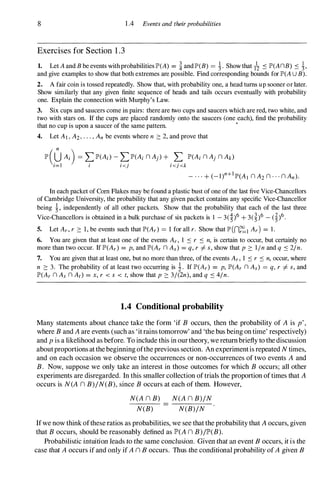
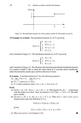
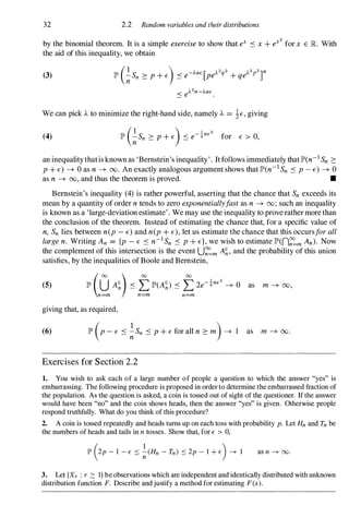
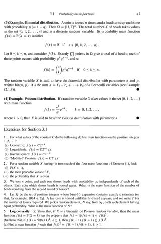
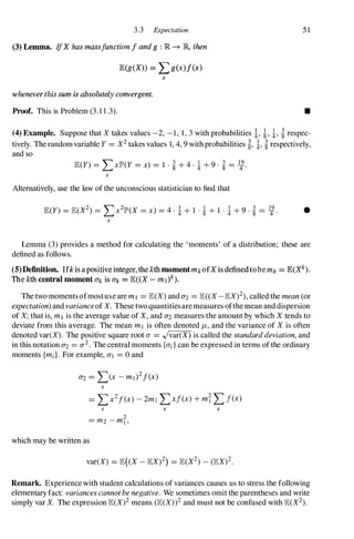
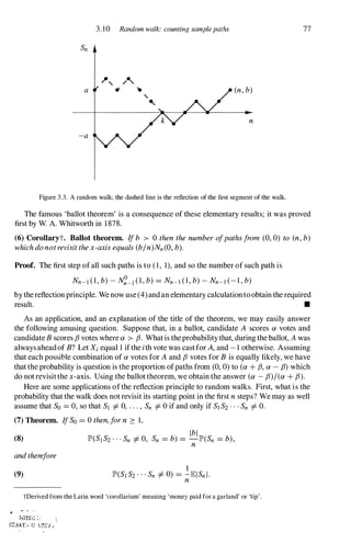
![2. 1 Random variables 27
Fx(x)
•
3 •
4'
1
4'
1 2 x
Figure 2.1. The distribution function Fx of the random variable X of Examples (1) and (5).
Afterthe experiment is doneandthe outcome W E Qis known, a randomvariable X : Q �
� takes some value. In general this numerical value is more likely to lie in certain subsets
of � than in certain others, depending on the probability space (Q, :F, JP') and the function X
itself. We wish to be able to describe the distribution of the likelihoods of possible values of
X. Example (1) above suggests that we might do this through the function f : � � [0, 1]
defined by
f(x) =probability that X is equal to x,
but this turns out to be inappropriate in general. Rather, we use the distribution function
F : � � � defined by
F(x) =probability that X does not exceed x.
More rigorously, this is
(2) F(x) =JP'(A(x))
where A(x) <; Q is given by A(x) ={w E Q : X (w) S x}. However, JP' is a function on the
collection :F of events; we cannot discuss JP'(A(x)) unless A(x) belongs to :F, and so we are
led to the following definition.
(3) Definition. A random variable is a function X : Q � R withthe property that {w E n :
X(w) ::s x} E :r for each x E R. Such a fnnction is said to be F-measurable.
If you so desire, you may pay no attention to the technical condition in the definition
and think of random variables simply as functions mappingQ into R We shall always use
upper-case letters, such as X, Y, and Z, to represent generic random variables, whilst lower
case letters, such as x, y, and z, will be used to represent possible numerical values of these
variables. Do not confuse this notation in your written work.
Every random variable has a distribution function, given by (2); distribution functions are
very important and useful.
(4) Definition. The distribution function of a random variable X is the function F : lR �
[0, l] given by F(x) = JP'(X � x).
This is the obvious abbreviation of equation (2). Events written as {w E Q : X (w) S x}
are commonly abbreviated to {w : X (w) S x} or {X S x}. We write Fx where it is necessary
to emphasize the role of X.](https://image.slidesharecdn.com/grimmettstirzaker-probabilityandrandomprocessesthirded2001-220507085451-bb31ac14/85/Grimmett-Stirzaker-Probability-and-Random-Processes-Third-Ed-2001-pdf-38-320.jpg)
![2.3 Discrete and continuous variables
2.3 Discrete and continuous variables
33
Much ofthe study of random variables is devoted to distribution functions, characterized by
Lemma (2. 1 .6). The general theory of distribution functions and their applications is quite
difficult and abstract and is best omitted at this stage. It relies on a rigorous treatment of
the construction of the Lebesgue-Stieltjes integral; this is sketched in Section 5.6. However,
things become much easier if we are prepared to restrict our attention to certain subclasses
of random variables specified by properties which make them tractable. We shall consider in
depth the collection of 'discrete' random variables and the collection of 'continuous' random
variables.
(1) Definition. The random variable X is called discrete ifit takes values in some countable
subset {Xl, X2 , . • • }, only, of R. The discrete random variable X has (probability) mass
function f : R -+ [0, 1] given by I(x) = P(X = x).
We shall see that the distribution function of a discrete variable has jump discontinuities
at the values Xl , X2 , . . . and is constant in between; such a distribution is called atomic. this
contrasts sharply with the other important class of distribution functions considered here.
(2) Definition. The random variable X is called continuous if its distribution function can
be expressed as
F(x) = L�feu) du x e R,
for some integrablefunction f : R -+ [0, (0) called the (probability) densityfunction ofX.
The distribution function of a continuous random variable is certainly continuous (actually
it is 'absolutely continuous'). For the moment we are concerned only with discrete variables
and continuous variables. There is another sort of random variable, called 'singular', for a
discussion ofwhich the reader should look elsewhere. A common example ofthis phenomenon
is based upontheCantorternary set (see Grimmettand Welsh 1986, orBillingsley 1995). Other
variables are 'mixtures' of discrete, continuous, and singular variables. Note that the word
'continuous' is a misnomer when used in this regard: in describing X as continuous, we are
referring to aproperty ofits distribution function rather than ofthe random variable (function)
X itself.
(3) Example. Discrete variables. The variables X and W of Example (2. 1 . 1) take values in
the sets {O, 1 , 2} and {O, 4} respectively; they are both discrete. •
(4) Example. Continuousvariables. A straight rod is flung down atrandom onto ahorizontal
plane and the angle w between the rod and true north is measured. The result is a number
in Q =[0, 2n). Never mind about F for the moment; we can suppose that F contains
all nice subsets of Q, including the collection of open subintervals such as (a, b), where
o S a < b < 2n. The implicit symmetry suggests the probability measure JP' which satisfies
JP'« a, b» = (b - a)/(2n); that is to say, the probability that the angle lies in some interval is
directly proportional to the length of the interval. Here are two random variables X and Y:
X(w) = w, Yew) = w2
.](https://image.slidesharecdn.com/grimmettstirzaker-probabilityandrandomprocessesthirded2001-220507085451-bb31ac14/85/Grimmett-Stirzaker-Probability-and-Random-Processes-Third-Ed-2001-pdf-44-320.jpg)
![34 2.3 Random variables and their distributions
Fx(x)
q
- 1 2]'[ x
Figure 2.3. The distribution function Fx of the random variable X in Example (5).
Notice that Y is a function of X in that Y = X2. The distribution functions of X and Y are
{O x < 0,
Fx(x) = x/(2]'[) O :s x < 2]'[,
1 x :::: 2]'[,
Fy(y) ={�/(2n)
To see this, let 0 :s x < 2]'[ and 0 :s y < 4]'[2. Then
Fx(x) = lP'({w E Q : 0 :s X(w) :s xl)
= lP'({w E Q : 0 :s w :s xl) =x/(2]'[),
Fy(y) = lP'({w : Yew) :s yl)
y :s 0,
O :s y < 4],[2,
y :::: 4]'[2.
= lP'({w : w2 :s yl) = lP'({w : O :s w :s .JYl) = lP'(X :s .JY)
=.JY/(2]'[).
The random variables X and Y are continuous because
where
Fx(x) = i�fx (u) du, Fy(y) =1:00fy (u) du,
fx (u) =
{ 1/(2]'[)
o
1
{ u- "2 /(4]'[)
fy (u) =
o
if 0 :s u :s 2]'[ ,
otherwise,
if 0 :s u :s 4],[2,
otherwise.
•
(5) Example. A random variable which is neither continuous nor discrete. A coin is
tossed, and a head turns up with probability p(= 1 -q). Ifa head turns up then arod is flung on
the ground and the angle measured as in Example (4). Then Q = {T}U{(H, x) : 0 :s x < 2]'[},
in the obvious notation. Let X : Q � lR be given by
X(T) = - 1 , X« H, x» = x.
The random variable X takes values in {- I }U [0, 2]'[) (see Figure 2.3 for a sketch of its
distribution function). We say that X is continuous with the exception of a 'point mass (or
atom) at - 1 ' . •](https://image.slidesharecdn.com/grimmettstirzaker-probabilityandrandomprocessesthirded2001-220507085451-bb31ac14/85/Grimmett-Stirzaker-Probability-and-Random-Processes-Third-Ed-2001-pdf-45-320.jpg)
![2.4 Worked examples 35
Exercises for Section 2.3
1. Let X be a random variable with distribution function F, and let a = (am : - 00 < m < 00)
be a strictly increasing sequence of real numbers satisfying a-m ---+ -00 and am ---+ 00 as m ---+ 00.
Define G(x) = lP'(X ::::: am) when am-I ::::: x < am, so that G is the distribution function ofa discrete
random variable. How does the function G behave as the sequence a is chosen in such a way that
sUPm lam -am-I I becomes smaller and smaller?
2. Let X be a random variable and let g : JR ---+ JR be continuous and strictly increasing. Show that
Y = g(X) is a random variable.
3. Let X be a random variable with distribution function
{0 if x ::::: 0,
lP'(X ::::: x } = x if O < x ::::: l ,
1 if x > l .
Let F be a distribution function which is continuous and strictly increasing. Show that Y = F-I (X)
is a random variable having distribution function F. Is it necessary that F be continuous and/or strictly
increasing?
4. Show that, if f and g are density functions, and 0 ::::: A ::::: 1 , then Af + (1 - A)g is a density. Is
the product fg a density function?
5. Which of the following are density functions? Find c and the corresponding distribution function
F for those that are.
{ cx-d x > 1 ,
(a) f(x) = .
o otherwIse.
(b) f(x) = ceX(l + ex)-2, x E JR.
2.4 Worked examples
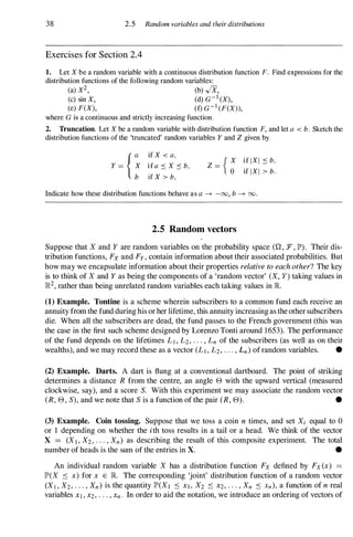
(1) Example. Darts. A dart is flung at a circular target of radius 3. We can think of the
hitting point as the outcome of a random experiment; we shall suppose for simplicity that the
player is guaranteed to hit the target somewhere. Setting the centre of the target at the origin
of ]R2, we see that the sample space of this experiment is
Q = {(x , y) : x2 + i < 9} .
Never mind about the collection :F of events. Let us suppose that, roughly speaking, the
probability that the dart lands in some region A is proportional to its area I A I . Thus
(2) JP'(A) = IA I/(9JT).
The scoring system is as follows. The target is partitioned by three concentric circles CI , C2,
and C3, centered at the origin with radii 1 , 2, and 3. These circles divide the target into three
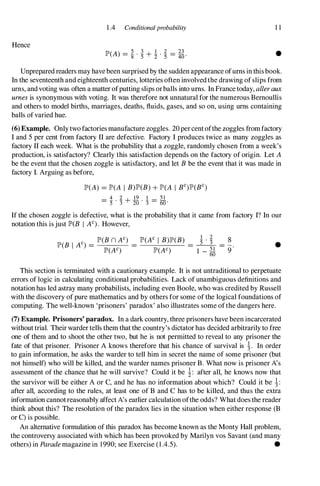
annuli A I , A2, and A3, where](https://image.slidesharecdn.com/grimmettstirzaker-probabilityandrandomprocessesthirded2001-220507085451-bb31ac14/85/Grimmett-Stirzaker-Probability-and-Random-Processes-Third-Ed-2001-pdf-46-320.jpg)
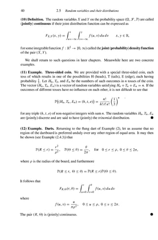
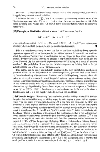
![2.4 Worked examples
Fy (r)
1
1 2 3 r
Figure 2.5. The distribution function Fy of Y in Example (3).
Fz(r)
1
I - p
-
2 3 4 r
Figure 2.6. The distribution function Fz of Z in Example (4).
This distribution function is sketched in Figure 2.5.
37
•
(4) Example. Continuation of (1). Now suppose that the player fails to hit the target with
fixed probability p; ifhe is successful then we suppose that the distribution ofthe hitting point
is described by equation (2). His score is specified as follows. If he hits the target then he
scores an amount equal to the distance between the hitting point and the centre; if he misses
then he scores 4. What is the distribution function of his score Z?
Solution. Clearly Z takes values in the interval [0, 4]. Use Lemma (1 .4.4) to see that
Fz(r) = lP'(Z � r)
= lP'(Z � r I hits target)lP'(hits target) + lP'(Z � r I misses target)lP'(misses target)
{,O if r < 0,
= (1 - p)Fy(r) if O � r < 4,
1 if r � 4,
where Fy is given in Example (3) (see Figure 2.6 for a sketch of Fz). •](https://image.slidesharecdn.com/grimmettstirzaker-probabilityandrandomprocessesthirded2001-220507085451-bb31ac14/85/Grimmett-Stirzaker-Probability-and-Random-Processes-Third-Ed-2001-pdf-48-320.jpg)
![2.5 Random vectors 39
real numbers: for vectors x = (Xl, X2, . . . , xn) and y = (Yl , Y2, . . . , Yn) we write x ::s y if
Xi ::s Yi for each i = 1 , 2, . . . , n.
(4)Deftnition. ThejointdistriootionfunctionofarandomvectorX = (Xl, X2 • • , . • Xn) on
the probability space (0 , :F, lP') is thefunction Fx : R.n -+ [0, 1] given by Fx(x) = lP'(X ::s x)
for x € R.n,
As before, the expression {X ::s x} is an abbreviation for the event {w E Q : X(w) ::s x}.
Joint distribution functions have properties similar to those ofordinary distribution functions.
For example, Lemma (2.1 .6) becomes the following.
(5) Lemma. Thejointdistributionfunction Fx,y o/the random vector (X, Y) has the/ollow
ingproperties:
(a) limx,y---+-oo Fx,y(x, y) =0, limx,y---+oo Fx,y(x, y) =1,
(b) If(XI, YI) ::s (X2, Y2) then FX,Y(XI , YI) ::s FX,Y(X2, Y2),
(c) Fx,y is continuous/rom above, in that
Fx,y(x + u, Y + v) --+ Fx,y(x, y) as u, v -I- 0.
We state this lemma for a random vector with only two components X and Y, but the
corresponding result for n components is valid also. The proof of the lemma is left as an
exercise. Rather more is true. It may be seen without great difficulty that
(6) lim Fx,y(x, y) =Fx(x) (=JP'(X ::s x»
y---+oo
and similarly
(7) lim Fx,y (x, y) =Fy(y) (=JP'(Y ::s y».
x---+oo ..
This more refined version ofpart (a) ofthe lemma tells us that we may recapture the individual
distribution functions of X and Y from a knowledge of their joint distribution function. The
converse is false: it is not generally possible to calculate Fx,y from a knowledge of Fx and
Fy alone. The functions Fx and Fy are called the 'marginal' distribution functions of Fx,y.
(8) Example. A schoolteacher asks each member of his or her class to flip a fair coin twice
and to record the outcomes. The diligent pupil D does this and records a pair (XD, YD) of
outcomes. Thelazypupil L flips the coin only once andwritesdowntheresult twice, recording
thus a pair (XL, Yd where XL =h . Clearly XD, YD, XL, and YL are random variables with
the same distribution functions. However, the pairs (XD, YD) and (XL, h) have different
joint distribution functions. In particular, JP'(XD =YD =heads) =i since only one of the
four possible pairs of outcomes contains heads only, whereas JP'(XL =h =heads) =1. •
Once again there are two classes of random vectors which are particularly interesting: the
'discrete' and the 'continuous' .
(9) Definition. The random variables X and Y on the probability space (Q, :F, JP') are called
(jointly) discrete if the vector (X, Y) takes values in some countable subset of ]R2 only. The
jointly discrete random variables X, Y have joint (probability) mass function / : ]R2 --+
[0, 1] given by lex, y) =JP'(X =x, Y =y).](https://image.slidesharecdn.com/grimmettstirzaker-probabilityandrandomprocessesthirded2001-220507085451-bb31ac14/85/Grimmett-Stirzaker-Probability-and-Random-Processes-Third-Ed-2001-pdf-50-320.jpg)
![42 2.6 Random variables and their distributions
(1) Example. Gambler's ruin revisited. The gambler of Example (1 .7.4) eventually won
his Jaguar after a long period devoted to tossing coins, and he has now decided to save up
for a yacht. His bank manager has suggested that, in order to speed things up, the stake on
each gamble should not remain constant but should vary as a certain prescribed function of
the gambler's current fortune. The gambler would like to calculate the chance of winning the
yacht in advance of embarking on the project, but he finds himself incapable of doing so.
Fortunately, he has kept a record ofthe extremely long sequence ofheads and tails encoun
tered in his successful play for the Jaguar. He calculates his sequence ofhypothetical fortunes
based on this information, until the point when this fortune reaches either zero or the price of
the yacht. He then starts again, and continues to repeat the procedure until he has completed
it a total of N times, say. He estimates the probability that he will actually win the yacht by
the proportion of the N calculations which result in success.
Can you see why this method will make him overconfident? He might do better to retoss
� �m. •
(2) Example. A dam. It is proposed to build a dam in order to regulate the water supply,
and in particular to prevent seasonal flooding downstream. How high should the dam be?
Dams are expensive to construct, and some compromise between cost and risk is necessary.
It is decided to build a dam which is just high enough to ensure that the chance of a flood
of some given extent within ten years is less than 10-2, say. No one knows' exactly how
high such a dam need be, and a young probabilist proposes the following scheme. Through
examination of existing records of rainfall and water demand we may arrive at an acceptable
model for the pattern of supply and demand. This model includes, for example, estimates for
the distributions of rainfall on successive days over long periods. With the aid of a computer,
the 'real world' situation is simulated many times in order to study the likely consequences
of building dams of various heights. In this way we may arrive at an accurate estimate of the
height required. •
(3) Example. Integration. Let g : [0, 1] � [0, 1] be a continuous but nowhere differentiable
function. How may we calculate its integral I =Jd g(x) dx? The following experimental
technique is known as the 'hit or miss Monte Carlo technique' .
Let (X, Y) be a random vector having the uniform distribution on the unit square. That is,
we assume that lP'((X, Y) E A) =IAI, the area of A, for any nice subset A ofthe unit square
[0, 1P; we leave the assumption of niceness somewhat up in the air for the moment, and shall
return to such matters in Chapter 4. We declare (X, Y) to be 'successful' if Y S g(X). The
chance that (X, Y) is successful equals I, the area under the curve y =g(x). We now repeat
this experiment a large number N of times, and calculate the proportion of times that the
experiment is successful. Following the law of averages, Theorem (2.2. 1), we may use this
value as an estimate of I.
Clearly it is desirable to know the accuracy of this estimate. This is a harder problem to
which we shall return later. •
Simulation is a dangerous game, and great caution is required in interpreting the results.
There are two major reasons for this. First, a computer simulation is limited by the degree
to which its so-called 'pseudo-random number generator' may be trusted. It has been said
for example that the summon-according-to-birthday principle of conscription to the United
States armed forces may have been marred by a pseudo-random number generator with a bias](https://image.slidesharecdn.com/grimmettstirzaker-probabilityandrandomprocessesthirded2001-220507085451-bb31ac14/85/Grimmett-Stirzaker-Probability-and-Random-Processes-Third-Ed-2001-pdf-53-320.jpg)
![3
Discrete random variables
Summary. The distribution of a discrete random variable may be specified via
its probability mass function. The key notion of independence for discrete
random variables is introduced. The concept of expectation, or mean value,
is defined for discrete variables, leading to a definition of the variance and the
moments of a discrete random variable. Joint distributions, conditional distri
butions, and conditional expectation are introduced, together with the ideas of
covariance and correlation. The Cauchy-Schwarz inequality is presented. The
analysis ofsums ofrandom variables leads to the convolution formulafor mass
functions. Random walks are studied in some depth, including the reflection
principle, the ballot theorem, the hitting time theorem, and the arc sine laws
for visits to the origin and for sojourn times.
3.1 Probability mass functions
Recall that a random variable X is discrete if it takes values only in some countable set
{Xl, X2, . . . }. Its distribution function F(x) =JP'(X :s x) is ajump function; just as important
as its distribution function is its mass function.
(1) Definition. The (probability) mass fnnctiontof a discrete random variable X is the
function f : R --* [0, 1] given by I(x) = JP'(X = x).
The distribution and mass functions are related by
i:x,::::x
I(x) =F(x) - lim F(y).
ytx
(2) Lemma. Theprobability massfunction I : IR --* [0, 1] satisfies:
(a) the set olx such that I(x) I- 0 is countable,
(b) Li I(Xi) =1, where Xl, X2, . . . are the values olx such that I(x) I- O.
Proof. The proof is obvious.
This lemma characterizes probability mass functions.
tSome refer loosely to the mass function of X as its distribution.
•](https://image.slidesharecdn.com/grimmettstirzaker-probabilityandrandomprocessesthirded2001-220507085451-bb31ac14/85/Grimmett-Stirzaker-Probability-and-Random-Processes-Third-Ed-2001-pdf-57-320.jpg)
![3.3 Expectation
However,
�lP'(Axn By) =lP'(Axn (yBy)) =lP'(Ax n Q) =lP'(Ax)
and similarly LxlP'(Axn By) =lP'(By),which gives
JE(aX + bY) =LaxLlP'(Axn By)+ LbyLlP'(Ax n By)
x y
x y
y x
53
=aJE(X) + bJE(Y). •
Remark. It is not in general true that JE(XY) is the same as JE(X)JE(Y).
(9) Lemma. IfX and Y are independent then JE(XY) =JE(X)JE(Y).
Proof. Let Axand Bybe as in the proof of (8). Then
and so
XY =LxyIAxnBy
x,y
JE(XY) =LxylP'(Ax)lP'(By) by independence
x,y
=LxlP'(Ax)LylP'(By) =JE(X)JE(Y).
x y
(10) Definition. X and Y are called uncorrelated if JE(XY) =JE(X)JE(Y).
•
Lemma (9) asserts that independent variables are uncorrelated. The converse is not true,
as Problem (3. 1 1 . 16) indicates.
(11) Theorem. For random variables X and Y,
(a) var(aX) =a2 var(X) for a E R,
(b) var(X + Y) =var(X) + var(y) ifX and Y are uncorrelated.
Proof. (a) Using the linearity of JE,
var(aX) =JE{(aX - JE(aX»2} =JE{a2(X - JEX)2}
=a2JE{(X - JEX)2} =a2 var(X).
(b) We have when X and Y are uncorrelated that
var(X + Y) =JE{(X + Y - JE(X + Y»)2
}
=JE[(X - JEX)2 + 2(XY - JE(X)JE(Y») + (Y _ JEy)2]
=var(X) + 2[JE(XY) - JE(X)JE(y)] + var(Y)
=var(X) + var(Y). •](https://image.slidesharecdn.com/grimmettstirzaker-probabilityandrandomprocessesthirded2001-220507085451-bb31ac14/85/Grimmett-Stirzaker-Probability-and-Random-Processes-Third-Ed-2001-pdf-64-320.jpg)
![56 3.4 Discrete random variables
3.4 Indicators and matching
This section contains light entertainment, in the guise of some illustrations of the uses of
indicator functions. These were defined in Example (2. 1 .9) and have appeared occasionally
since. Recall that
and lElA =JP>(A).
{ I if W E A,
IA (W) = 0
if w E AC,
(1) Example. Proofs of Lemma (1.3.4c, d). Note that
IAUB =1 - I(AUB)C =1 - IAcnBc
=1 - IAc lBc =1 - (1 - IA)(1 - IB)
=IA + IB - IAIB·
Take expectations to obtain
JP>(AU B) =JP>(A) + JP>(B) - JP>(A n B).
More generally, if B =U7=1 Ai then
n
IB =1 - n(1 - IA, );
i=1
multiply this out and take expectations to obtain
(2) JP>(0Ai) =�JP>(Ai) - �JP>(Ai n Aj) + . . . + (_l)n+IJP>(AI n · · · n An)·
1=1 1 I <j
This very useful identity is known as the inclusion-exclusionformula. •
(3) Example. Matching problem. A number of melodramatic applications of (2) are avail
able, of which the following is typical. A secretary types n different letters together with
matching envelopes, drops the pile down the stairs, and then places the letters randomly in
the envelopes. Each arrangementis equally likely, and we ask for the probability that exactly
r are in their correct envelopes. Rather than using (2), we shall proceed directly by way of
indicator functions. (Another approach is presented in Exercise (3.4.9).)
Solution. Let LI, L2, . . . , Ln denote the letters. Call a letter good ifit is correctly addressed
and bad otherwise; write X for the number of good letters. Let Ai be the event that Li is
good, and let Ii be the indicator function of Ai. Let j] , . . . , jr, kr+1 , . . . , kn be a permutation
of the numbers 1 , 2, . . . , n, and define
(4) S =LIh . . . Ijr (1 - hr+1 ) . . . (1 - hn )
rr](https://image.slidesharecdn.com/grimmettstirzaker-probabilityandrandomprocessesthirded2001-220507085451-bb31ac14/85/Grimmett-Stirzaker-Probability-and-Random-Processes-Third-Ed-2001-pdf-67-320.jpg)
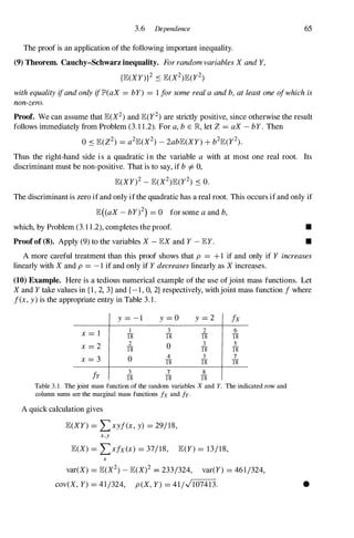
![3.6 Dependence 63
variable is its distribution function, so the study of, say, a pair of random variables is based
on its 'joint' distribution function and mass function.
(2) Definition. The Joint distribution function F : )R2 -* [0, 1] of X and Y, where X and
Y are discrete variables, is given by
F(x, y) = P(X :s x and Y :s y).
Theirjoint mass function I : R2 ... [0, 1] is given by
f(x, y) = P(X = x and Y = y).
Joint distribution functions and joint mass functions of larger collections of variables are
defined similarly. The functions F and I can be characterized in much the same way (Lemmas
(2. 1 .6) and (3 . 1 .2» as the corresponding functions of a single variable.We omit the details.
We write FX,Y and Ix,Y when we need to stress the role of Xand Y. You may think of the
joint mass function in the following way. If Ax = {X = x} and By = {Y = y}, then
I(x, y) = lP'(Ax n By).
The definition of independence can now be reformulated in a lemma.
(3) Lemma. The discrete random variables X and Y are independent ifandonly if
(4) /x,y(x, y) = Ix(x)/y(y) forall x. y E R.
More generally, X and Y are independent ifandonly if/x,y(x, y) Can belactorized as the
product g(x)h(y) ofafunction 01x alone and a function 01y alone.
Proof. This is Problem (3. 1 1 . 1 ). •
Suppose that X and Y have joint mass function Ix,Y and we wish to check whether or
not (4) holds. First we need to calculate the marginal mass functions Ix and Iy from our
knowledge of Ix,Y. These are found in the following way:
Ix (x) = lP'(X= x) = lP'(U({X= x} n {Y = yn)
y
= LlP'(X = x, Y = y) = L/x,y(x, y),
y y
and similarly Iy (y) = Lx Ix,Y(x, y). Having found the marginals, it is a trivial matter to
see whether (4) holds or not.
Remark. We stress thatthe factorization (4) must hold for all x and y in orderthat Xand Y
be independent.
(5) Example. Calculation ofmarginaIs. In Example (3.2.2) we encountered a pair X, Y of
variables with a joint mass function
aXf3Y
I(x, y) = __ e-a-fJ " 0 1 2
lor x, y = , , , . . .
x ! y !](https://image.slidesharecdn.com/grimmettstirzaker-probabilityandrandomprocessesthirded2001-220507085451-bb31ac14/85/Grimmett-Stirzaker-Probability-and-Random-Processes-Third-Ed-2001-pdf-74-320.jpg)
![64 3.6 Discrete random variables
where ex, f3 > O. The marginal mass function of X is
and so Xhas the Poisson distribution withparameterex . Similarly Y has the Poisson distribution
with parameter f3. It is easy to check that (4) holds, whence X and Y are independent. •
For any discrete pair X, Y, a real function g(X, Y) is a random variable. We shall often
need to find its expectation. To avoid explicit calculation of its mass function, we shall use
the following more general form ofthe law of the unconscious statistician, Lemma (3.3.3).
(6) Lemma. lE(g(X, Y)) =Lx,yg(x, y)fx,Y(x, y).
Proof. As for Lemma (3.3.3). •
For example, lE(XY) =Lx,yxyfx,Y(x, y). This formula is particularly useful to statisti
cians who may need to find simple ways of explaining dependence to laymen. For instance,
suppose thatthe government wishes to announce that the dependence between defence spend
ing and the cost of living is very small. It should not publish an estimate of the joint mass
function unless its object is obfuscation alone. Most members of the public would prefer to
find that this dependence can be represented in terms of a single number on a prescribed scale.
Towards this end we make the following definitiont.
(7) Definition. The covariance of X and Y is
cov(X, Y) =lE[(X - lEX) (Y - lEY)].
The correlation (coefficient) of X and Y is
cov(X, Y)
P(X, Y) =--;===;:;:;:;::=:===;:�
,Jvar(X) . var(Y)
as long as the variances are non-zero.
Note that the concept ofcovariance generalizes that ofvariance in that cov(X, X) =var(X).
Expanding the covariance gives
cov(X, Y) =lE(XY) - lE(X)lE(Y) .
Remember, Definition (3.3. 10), that X and Y are called uncorrelatedi fcov(X, Y ) =O. Also,
independent variables are always uncorrelated, although the converse is not true. Covariance
itself is not a satisfactory measure of dependence because the scale of values which cov(X, Y)
may take contains no points which are clearly interpretable in terms ofthe relationship between
X and Y. The following lemma shows that this is not the case for correlations.
(8) Lemma. The correlation coefficient p satisfies Ip(X, Y)I S 1 with equality ifand only if
JP'(aX + bY = c) =1 for some a, b, c E R
tThe concepts and terminology in this definition were formulated by Francis Galton in the late 1880s.](https://image.slidesharecdn.com/grimmettstirzaker-probabilityandrandomprocessesthirded2001-220507085451-bb31ac14/85/Grimmett-Stirzaker-Probability-and-Random-Processes-Third-Ed-2001-pdf-75-320.jpg)
![66 3.6 Discrete random variables
Exercises for Section 3.6
1. Show that the collection of random variables on a given probability space and having finite
variance forms a vector space over the reals.
2. Find the marginal mass functions of the multinomial distribution of Exercise (3.5.1).
3. Let X and Y be discrete random variables with joint mass function
c
f(x, y) = ,
(x + y - 1)(x + y)(x + y + 1)
x, y = 1, 2, 3, . . . .
Find the marginal mass functions of X and Y, calculate C, and also the covariance of X and Y.
4. Let X and Y be discrete random variables with mean 0, variance 1, and covariance p . Show that
JE (max{X
2, y2}) ::::: 1 + J1=P2.
5. Mutual information. Let X and Y be discrete random variables with joint mass function f.
(a) Show that JE(log fx (X» :::: JE(log fy (X».
(b) Show that the mutual information
I - JE (10 { f(X, Y) })
- g
fx(X)fy (Y)
satisfies I :::: 0, with equality if and only if X and Y are independent.
6. Voter paradox. Let X, Y, Z be discrete random variables with the property that their values are
distinct with probability 1. Let a = JP'(X > Y), b = JP'(Y > Z), c = JP'(Z > X).
(a) Show that min{a, b, c} ::::: �, and give an example where this bound is attained.
(b) Show that, if X, Y, Z are independent and identically distributed, then a = b = c = �.
(c) Find min{a, b, c} and sUPp min{a, b, c} when JP'(X = 0) = 1, and Y, Z are independent with
JP'(Z = 1) = JP'(Y = -1) = p, JP'(Z = -2) = JP'(Y = 2) = 1 - p. Here, sUPp denotes the
supremum as p varies over [0, 1].
[Part (a) is related to the observation that, in an election, it is possible for more than half of the voters
to prefer candidate A to candidate B, more than half B to C, and more than half C to A.]
7. Benford's distribution, or the law of anomalous numbers. If one picks a numerical entry at
random from an almanac, or the annual accounts of a corporation, the first two significant digits, X,
Y, are found to have approximately thejoint mass function
f(x, y) = 10glO (1 + lO
x
1
+ y
) ' 1 ::::: x ::::: 9, 0 ::::: y ::::: 9.
Find the mass function of X and an approximation to its mean. [A heuristic explanation for this
phenomenon may be found in the second of Feller's volumes (197 1 ).]
8. Let X and Y have joint mass function
. k _
c(j + k)aHk
f(} , ) - . ' k' ' j, k :::: 0,
} . .
where a is a constant. Find c, JP'(X = j), JP'(X + Y = r), and JE(X).](https://image.slidesharecdn.com/grimmettstirzaker-probabilityandrandomprocessesthirded2001-220507085451-bb31ac14/85/Grimmett-Stirzaker-Probability-and-Random-Processes-Third-Ed-2001-pdf-77-320.jpg)
![3.9 Simple random walk 7 1
Exercises for Section 3 . 8
1. Let X and Y be independent variables, X being equally likely to take any value in {O, 1 , . . . , m},
and Y similarly in {O, 1, . . . , n}. Find the mass function of Z = X + Y. The random variable Z is
said to have the trapezoidal distribution.
2. Let X and Y have the joint mass function
c
f(x, y) = ,
(x + y - l)(x + y)(x + y + 1)
x, y = 1 , 2, 3, . . . .
Find the mass functions of U = X + Y and V = X - Y.
3. Let X and Y be independent geometric random variables with respective parameters a and f3.
Show that
IP'(X + Y = z) = � {(l - f3)z-l - (1 - a)Z-l }.
a - f3
4. Let {Xr : 1 � r :::: n} be independent geometric random variables with parameter p. Show that
Z = L:�=l Xr has a negative binomial distribution. [Hint: No calculations are necessary.]
5. Pepys's problemt. Sam rolls 6n dice once; he needs at least n sixes. Isaac rolls 6(n + 1) dice;
he needs at least n + 1 sixes. Who is more likely to obtain the number of sixes he needs?
6. Let N be Poisson distributed with parameter A. Show that, for any function g such that the
expectations exist, IE(Ng(N)) = AIEg(N + 1). More generally, if S = L:�l Xr, where {Xr : r ::: O}
are independent identically distributed non-negative integer-valued random variables, show that
IE(Sg(S») = AIE(g(S + Xo)Xo) .
3.9 Simple random walk
Until now we have dealt largely with general theory; the final two sections of this chapter
may provide some lighter relief. One of the simplest random processes is so-called 'simple
random walk' :!:; this process arises in many ways, of which the following is traditional. A
gambler G plays the following game at the casino. The croupier tosses a (possibly biased)
coin repeatedly; each time heads appears, he gives G one franc, and each time tails appears
he takes one franc from G. Writing Sn for G's fortune after n tosses of the coin, we have
that Sn+l =Sn + Xn+l where Xn+l is a random variable taking the value 1 with some fixed
probability p and - 1 otherwise; furthermore, Xn+1 is assumed independent of the results of
all previous tosses. Thus
(1)
n
Sn =so + LX; ,
;=1
tPepys put a simple version of this problem to Newton in 1693, but was reluctant to accept the correct reply
he received.
tKarl Pearson coined the term 'random walk' in 1906, and (using a result of Rayleigh) demonstrated the
theorem that "the most likely place to find a drunken walker is somewhere near his starting point", empirical
verification of which is not hard to find.](https://image.slidesharecdn.com/grimmettstirzaker-probabilityandrandomprocessesthirded2001-220507085451-bb31ac14/85/Grimmett-Stirzaker-Probability-and-Random-Processes-Third-Ed-2001-pdf-82-320.jpg)
![72 3.9 Discrete random variables
so that Sn is obtained from the initial fortune So by the addition of. n independent random
variables. We are assuming herethatthere are no constraints on G's fortuneimposed externally,
such as that the game is terminated if his fortune is reduced to zero.
An alternative picture of 'simple random walk' involves the motion ofa particle-a particle
which inhabits the set of integers and which moves at each step either one step to the right,
with probability p, or one step to the left, the directions ofdifferent steps being independent of
each other. More complicated random walks arise when the steps of the particle are allowed
to have some general distribution on the integers, or the reals, so that the position Sn at time
n is given by (1) where the Xi are independent and identically distributed random variables
having some specified distribution function. Even greater generality is obtained by assuming
thatthe Xi take values in ]Rd for some d ::::: 1 , or even some vector space overthereal numbers.
Random walks may be used with some success in modelling various practical situations, such
as the numbers of cars in a toll queue at 5 minute intervals, the position of a pollen grain
suspended in fluid at 1 second intervals, or the value of the Dow-Jones index each Monday
morning. In each case, it may not be too bad a guess that the (n + l )th reading differs from the
nth by a random quantity which is independent ofpreviousjumps but has the same probability
distribution. The theory of random walks is a basic tool in the probabilist's kit, and we shall
concern ourselves here with 'simple random walk' only.
At any instant of time a particle inhabits one ofthe integer points of the real line. At time
o it starts from some specified point, and at each subsequent epoch of time 1 , 2, . . . it moves
from its current position to a new position according to the following law. With probability
p it moves one step to the right, and with probability q = 1 - P it moves one step to the left;
moves are independent of each other. The walk is called symmetric if p = q = !. Example
(1 .7.4) concerned a symmetric random walk with 'absorbing' barriers at the points 0 and N.
In general, let Sn denote the position of the particle after n moves, and set So = a. Then
(2)
n
Sn = a + LXi
i=!
where X! , X2 , . . . is a sequence of independent Bernoulli variables taking values +1 and - 1
(rather than +1 and 0 as before) with probabilities p and q .
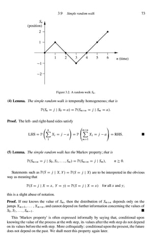
We record the motion of the particle as the sequence {en, Sn) : n ::::: O} of Cartesian
coordinates of points in the plane. This collection of points, joined by solid lines between
neighbours, is called the path of the particle. In the example shown in Figure 3.2, the particle
has visited the points 0, 1 , 0, - 1 , 0, 1 , 2 in succession. This representation has a confusing
aspect in that the direction of the particle's steps is parallel to the y-axis, whereas we have
previously been specifying the movement in the traditional way as to the right or to the left.
In future, any reference to the x-axis or the y-axis will pertain to a diagram of its path as
exemplified by Figure 3.2.
The sequence (2) ofpartial sums has three important properties.
(3) Lemma. The simple random walk is spatially homogeneous; thatis
JP'(Sn = j I So = a) = JP'(Sn = j + b I So = a + b).
Proof. Both sides equal JP'(L� Xi = j - a). •](https://image.slidesharecdn.com/grimmettstirzaker-probabilityandrandomprocessesthirded2001-220507085451-bb31ac14/85/Grimmett-Stirzaker-Probability-and-Random-Processes-Third-Ed-2001-pdf-83-320.jpg)
![74 3.9 Discrete random variables
(6) Example. Absorbing barriers. Let us revisit Example (1 .7.4) for general values of p.
Equation ( 1 .7.5) gives us the following difference equation for the probabilities {Pk} where
Pk is the probability of ultimate ruin starting from k:
(7) Pk = p . PHI + q . Pk-I if 1 S k S N - 1
with boundary conditions Po = 1 , PN = O. The solution of such a difference equation
proceeds as follows. Look for a solution of the form Pk = (Jk. Substitute this into (7) and
cancel out the power (Jk-I to obtain p(J2
- (J + q = 0, which has roots (JI = 1 , (J2 = q/p. If
P =1= � then these roots are distinct and the general solution of (7) is Pk = AI (J� + A2(J� for
arbitrary constants A l and A2. Use the boundary conditions to obtain
(q/p)k _ (q/p)N
Pk =
1 _ (q/p)N
If P = � then (JI = (J2 = 1 and the general solution to (7) is Pk = A l + A2k. Use the
boundary conditions to obtain Pk = 1 - (k/N).
A more complicated equation is obtained for the mean number Dk of steps before the
particle hits one of the absorbing barriers, starting from k. In this case we use conditional
expectations and (3.7.4) to find that
(8)
with the boundary conditions Do = DN = O. Try solving this; you need to find a general so
lution and a particular solution, as in the solution of second-orderlineardifferential equations.
This answer is
(9) Dk = { q �P
[k - N (;��::;�)] if P =1= �,
keN - k) if P = �.
•
(10) Example. Retaining barriers. In Example ( 1 .7.4), suppose that the Jaguar buyer has
a rich uncle who will guarantee all his losses. Then the random walk does not end when the
particle hits zero, although it cannot visit a negative integer. Instead lP'(Sn+l = 0 I Sn = 0) = q
and lP'(Sn+1 = 1 I Sn =0) = p. The origin is said to have a 'retaining' barrier (sometimes
called 'reflecting' ).
What now is the expected duration of the game? The mean duration Fk , starting from k,
satisfies the same difference equation (8) as before but subjectto different boundary conditions.
We leave it as an exercise to show that the boundary conditions are FN = 0, pFo = 1 + pFI,
and hence to find Fk. •
In such examples the techniques of 'conditioning' are supremely useful. The idea is that
in order to calculate a probability lP'(A) or expectation JE(Y) we condition either on some
partition of Q (and use Lemma ( 1 .4.4» or on the outcome of some random variable (and use
Theorem (3.7.4) or the forthcoming Theorem (4.6.5» . In this section this technique yielded
the difference equations (7) and (8). In later sections the same idea will yield differential
equations, integral equations, and functional equations, some of which can be solved.](https://image.slidesharecdn.com/grimmettstirzaker-probabilityandrandomprocessesthirded2001-220507085451-bb31ac14/85/Grimmett-Stirzaker-Probability-and-Random-Processes-Third-Ed-2001-pdf-85-320.jpg)
![3.10 Random walk: counting sample paths
Exercises for Section 3.9
75
1. Let Tbe the time which elapses before a simple random walk is absorbed ateither ofthe absorbing
barriers at O and N, having started at k where 0 :s k :s N. Show that IP'(T < 00) = 1 and JE(Tk
) < 00
for all k :::: 1 .
2. For simple random walk S with absorbing barriers at 0 and N, let W be the event that the particle
is absorbed at 0 rather than at N, and let Pk = IP'(W I So = k). Show that, if the particle starts at
k where 0 < k < N, the conditional probability that the first step is rightwards, given W, equals
PPk+1 /Pk· Deduce that the mean duration h of the walk, conditional on W, satisfies the equation
PPk+1 Jk+l - Pkh + (Pk - PPk+] ) Jk-I = -Pk . for 0 < k < N.
Show that we may take as boundary condition JO = O. Find h in the symmetric case, when P = �.
3. With the notation of Exercise (2), suppose further that at any step the particle may remain where
it is with probability r where P + q + r = 1 . Show that h satisfies
PPk+l Jk+I - (1 - r)Pkh + qPk-I Jk-l = -Pk
and that, when p = q/P I=- 1,
h = _
I _ . 1
{k(pk + pN) _
2NpN(I - pk)
} .
P _ q pk _ pN 1 _ pN
4. Problem ofthe points. A coin is tossed repeatedly, heads turning up with probability P on each
toss. Player A wins the game if m heads appear before n tails have appeared, and player B wins
otherwise. Let Pmn be the probability that A wins the game. Set up a difference equation for the pmn .
What are the boundary conditions?
5. Consider a simple random walk on the set {O, 1, 2, . . . , N} in which each step is to the right with
probability P or to the left with probability q = 1 - p. Absorbing barriers are placed at 0 and N.
Show that the number X of positive steps of the walk before absorption satisfies
where Dk is the mean number of steps until absorption and Pk is the probability of absorption at O.
6. (a) "Millionaires should always gamble, poor men never" [J. M. Keynes].
(b) "If I wanted to gamble, I would buy a casino" [Po Getty].
(c) "That the chance of gain is naturally overvalued, we may learn from the universal success of
lotteries" [Adam Smith, 1776].
Discuss.
3.10 Random walk: counting sample paths
In the previous section, our principal technique was to condition on the first step of the walk
and then solve the ensuing difference equation. Another primitive but useful technique is
to count. Let XI , X2 , . . . be independent variables, each taking the values - 1 and 1 with
probabilities q = 1 - P and p, as before, and let
(1)
n
Sn = a + LX;
;=1](https://image.slidesharecdn.com/grimmettstirzaker-probabilityandrandomprocessesthirded2001-220507085451-bb31ac14/85/Grimmett-Stirzaker-Probability-and-Random-Processes-Third-Ed-2001-pdf-86-320.jpg)
![78 3.10 Discrete random variables
Proof. Suppose that So= 0 and Sn = b(> 0). The event in question occurs if and only ifthe
path of the random walk does not visit the x -axis in the time interval [1,n]. The number of
such paths is, by theballottheorem, (b/n)Nn(O,b),and each suchpathhas !(n+b)rightward
steps and !(n-b)leftward steps. Therefore
as required. A similar calculation is valid if b < O. •
Another feature of interest is the maximum value attained by the random walk. We write
Mn = max{Sj : 0 S i S n} for the maximum value up to time n, and shall suppose that
So = 0, so that Mn � O. Clearly Mn � Sn,and the first part of the next theorem is therefore
trivial.
(10) Theorem. SupposethatSo = O. Then,for r � 1,
{ lP'(Sn = b) if b � r,
(11) lP'(Mn � r, Sn = b) =
(q/py-blP'(Sn = 2r _ b) if b < r.
It follows that, for r � 1,
r-l
(12) lP'(Mn � r) = lP'(Sn � r) + L (q/py-blP'(Sn = 2r -b)
b=-oo
00
= lP'(Sn =r) + L [1 +(q/p)c-r]lP'(Sn =c),
c=r+l
yielding in the symmetric case when p= q = !that
(13) lP'(Mn � r) = 2lP'(Sn � r +1) +lP'(Sn = r),
which is easily expressed in terms of the binomial distribution.
Proof of (10). We may assume that r � 1and b < r. Let N�(0, b)be the number of paths
from (0, 0) to (n,b) which include some point having height r, which is to say some point
(i, r) with 0 < i < n; for such a path Jr , let (in, r) be the earliest such point. We may
reflect the segment of the path with in S x S nin the line y = r to obtain a path Jr
'
joining
(0, 0) to (n,2r -b). Any such path Jr
'
is obtained thus from a unique path Jr , and therefore
N�(0, b) = Nn(0, 2r -b). It follows as required that
lP'(Mn � r, Sn = b) = N�(O,b)p�(n+b)q�(n-b)
= (q/py-bNn(O,2r _ b)p�(n+2r-b)q�(n-2r+b)
= (q/py-blP'(Sn = 2r -b). •](https://image.slidesharecdn.com/grimmettstirzaker-probabilityandrandomprocessesthirded2001-220507085451-bb31ac14/85/Grimmett-Stirzaker-Probability-and-Random-Processes-Third-Ed-2001-pdf-89-320.jpg)
![3.10 Random walk: counting samplepaths 79
What is the chance that the walk reaches a new maximum at a particular time? More
precisely, what is the probability that the walk, starting from 0,reaches the point b(> 0)for
the time time at the nth step? Writing fb(n)for this probability, we have that
fb(n) =lP'(Mn-l =Sn-l =b- 1, Sn =b)
=p[lP'(Mn-l :::: b- 1, Sn-l =b- 1) -lP'(Mn-l :::: b, Sn-l =b- 1)]
=p[lP'(Sn-l =b- 1) -(q/p)lP'(Sn-l =b+1)] by (11)
b
=-lP'(Sn =b)
n
by a simple calculation using (2). A similar conclusion may be reached if b < 0,and we
arrive at the following.
(14) Hitting time theorem. Theprobabilityfb(n) thatarandomwalkShitsthepointbfor
thefirsttimeatthenthstep,havingstartedfrom0,satisfies
(15)
Ibl
fb(n) =-lP'(Sn =b) if n :::: 1 .
n
The conclusion here has a close resemblance to that of the ballot theorem, and particularly
Theorem (7). This is no coincidence: a closer examination of the two results leads to another
technique for random walks, the technique of 'reversal' . If the first n steps of the original
random walk are
then the steps of the reversedwalk, denoted by 0,Tl,... ,Tn,are given by
{O,Tl,T2,... ,Tn} =[0,Xn,Xn +Xn-l,... ,�Xi).
Draw a diagram to see how the two walks correspond to each other. The Xi are independent
and identically distributed, and it follows that the two walks have identical distributions even
if p=1= !. Notice that the addition of an extra step to the original walk may change everystep
of the reversed walk.
Now, theoriginalwalk satisfies Sn =b(> 0)and SlS2...Sn =1=0ifand only ifthereversed
walk satisfied Tn = band Tn -Tn-i =Xl +...+Xi > 0for all i :::: 1,which is to say that
the first visit of the reversed walk to the point btakes place at time n. Therefore
(16)
This is the 'coincidence' remarked above; a similar argument is valid if b < O. The technique
of reversal has other applications. For example, let /Lb be the mean number of visits of the
walk to the point bbefore it returns to its starting point. If So = 0then, by (16),
00 00
(17) /Lb =LlP'(SIS2'" Sn =1=0,Sn =b) =Lfb(n) =lP'(Sn =bfor some n),
n=l n=l](https://image.slidesharecdn.com/grimmettstirzaker-probabilityandrandomprocessesthirded2001-220507085451-bb31ac14/85/Grimmett-Stirzaker-Probability-and-Random-Processes-Third-Ed-2001-pdf-90-320.jpg)
![80 3.10 Discrete random variables
the probability of ultimately visiting b. This leads to the following result.
(18) Theorem. Ifp =! andSo =0,foranyb(=f. 0)themeannumberI1b ofvisitsofthe
walktothepointbbeforereturningtotheoriginequals1.
Proof. Let fb =JP>(Sn =bfor some n ::: 0). We have, by conditioning on the value of Sl,
that fb =!(fb+1 + fb-l)for b > 0, with boundary condition fa =1 . The solution of this
difference equation is fb = Ab + B for constants Aand B. The unique such solution lying
in [0, 1] with fa =1 is given by fb =1 for all b ::: O. By symmetry, fb =1 for b S O.
However, fb =I1bfor b=f.0,and the claim follows. •
'The truly amazing implications of this result appear best in the language of fair games. A
perfect coin is tossed until the first equalization ofthe accumulated numbers ofheads and tails.
The gambler receives one penny for every time thatthe accumulated number ofheads exceeds
the accumulated number of tails by m. The"fairentrancefee"equals1 independentlyofm.'
(Feller 1968,p. 367).
We conclude with two celebrated properties of the symmetric random walk.
(19) Theorem. Arc sine lawforlast visit to the origin. Supposethatp=! andSo=O. The
probabilitythatthelastvisitto0uptotime2noccurredattime2kisJP>(S2k =0)JP>(S2n-2k =0).
In advance ofproving this, we notesomeconsequences. Writing a2n(2k)fortheprobability
referred to in the theorem, it follows from the theorem that a2n(2k) =U2kU2n-2kwhere
(2k) -2k
U2k =JP>(S2k =0) = k 2 .
In order to understand the behaviour of U2kfor large values of k,we use Stirling's formula:
(20)
which is to say that the ratio ofthe left-hand side to the right-hand side tends to 1as n -+ 00.
Applying this formula, we obtain that U2k '" 1/...fi[kas k -+ 00. This gives rise to the
approximation
1
a2 (2k) '" -----r.::.:;==�
n - n../k(n -k),
valid for values of kwhich are close to neither 0nor n. With T2ndenoting the time ofthe last
visit to 0up to time 2n,it follows that
1 lxn 1 2
JP>(T2n < 2xn) � L '" du =-sin-1 ..jX,
- k n../k(n-k) u=on"/u(n-u) n
sxn
which is to say that T2n/(2n)has adistribution function which is approximately (2/n)sin-1 ..jX
when nis sufficiently large. We have proved a limit theorem.
The arc sine law is rather surprising. One may think that, in a long run of 2ntosses of a
fair coin, the epochs of time at which there have appeared equal numbers of heads and tails
should appear rather frequently. On the contrary, there is for example probability ! that no
such epoch arrived in the final ntosses, and indeed probability approximately !that no such
epoch occurred after the first !n tosses. One may think that, in a long run of 2ntosses of a](https://image.slidesharecdn.com/grimmettstirzaker-probabilityandrandomprocessesthirded2001-220507085451-bb31ac14/85/Grimmett-Stirzaker-Probability-and-Random-Processes-Third-Ed-2001-pdf-91-320.jpg)
![3.10 Random walk: counting samplepaths 8 1
fair coin, the last time at which the numbers of heads and tails were equal tends to be close to
the end. On the contrary, the distribution of this time is symmetric around the midpoint.
How much time does a symmetric random walk spend to the right of the origin? More
precisely, for how many values of k satisfying 0 :'S k :'S 2n is it the case that Sk > O?
Intuitively, one might expect the answer to be around nwith large probability, but the truth is
quite different. With large probability, the proportion of time spent to the right (or to the left)
of the origin is near to 0or to 1,but not near to !. That is to say, in a long sequence of tosses
of a fair coin, there is large probability that one face (either heads or tails) will lead the other
for a disproportionate amount of time.
(21) Theorem. Arc sine law for sojourn times. Supposethatp = ! andSo = O. The
probabilitythatthewalkspendsexactly2kintervalsa/time,uptotime2n, totherighta/the
originequalsJP'(S2k =0)JP'(S2n-2k =0).
We say that the interval (k,k+ 1) is spent to the right of the origin if either Sk > 0or
Sk+l > O. It is clear that the number of such intervals is even if the total number of steps is
even. The conclusion of this theorem is most striking. First, the answer is the same as that
of Theorem (19). Secondly, by the calculations following (19)we have that the probability
that the walk spends 2xn units of time or less to the right of the origin is approximately
(2In)sin-1 ,JX.
Proofof (19). The probability in question is
(){2n(2k) =JP'(S2k =0)JP'(S2k+lS2k+2...S2n =f.0 I S2k =0)
=JP'(S2k =O)JP'(SIS2...S2n-2k =f.0).
Now, setting m =n-k,we have by (8) that
(22)
=2(�)2mt[( 2m- l )_ (2m- l)]
2 m+k- l m+k
k=l
=2(�rm Cm
m
- 1)
(2m)(1)2m
= m "2 =JP'(S2m =0).
In passing, note the proof in (22)that
(23)
for the simple symmetric random walk.
•
Proof of (21). Let fhn(2k)be the probability in question, and write U2m =JP'(S2m = 0) as
before. We are claiming that, for all m � 1,
(24) f32m(2k) =U2kU2m-2k if O:'Sk :'Sm.](https://image.slidesharecdn.com/grimmettstirzaker-probabilityandrandomprocessesthirded2001-220507085451-bb31ac14/85/Grimmett-Stirzaker-Probability-and-Random-Processes-Third-Ed-2001-pdf-92-320.jpg)
![82 3.10 Discrete random variables
First,
lP'(S]S2···S2m > 0) =lP'(S] =1, S2 2: 1,... , S2m 2: 1)
=ilP'(S] 2:0, S2 2:0,... , S2m-] 2:0),
where the second line follows by considering the walk S] - 1,S2 - 1,... ,S2m - 1. Now
S2m-] is an odd number, so that S2m-] 2:0implies that S2m 2:0also. Thus
yielding by (23)that
and (24)follows for k =m, and therefore for k=0also by symmetry.
Let nbe a positive integer, and let Tbe the time ofthe first return ofthe walk to the origin.
If S2n =0then T S 2n;the probability mass function hr =lP'(T =2r)satisfies
n n
lP'(S2n =0) =LlP'(S2n =0 I T =2r)lP'(T =2r) =LlP'(S2n-2r =O)lP'(T=2r),
r=]
which is to say that
(25)
n
U2n =LU2n-2rhr.
r=]
r=]
Let 1 S k S n - 1, and consider fhn(2k). The corresponding event entails that T =2r
for some rsatisfying 1 S r < n. The time interval (0, T)is spent entirely either to the right
or the left of the origin, and each possibility has probability i. Therefore,
k n-k
(26) /32n(2k) =LilP'(T =2r)fhn-2r(2k-2r)+LilP'(T =2r)/32n-2r(2k).
r=l r=]
We conclude the proofby using induction. Certainly (24)is valid for all kifm =1. Assume
(24)is valid for all kand all m < n.
From (26),
k n-k
/32n(2k) =i LhrU2k-2rU2n-2k+i LhrU2kU2n-2k-2r
r=] r=]
by (25),as required. •](https://image.slidesharecdn.com/grimmettstirzaker-probabilityandrandomprocessesthirded2001-220507085451-bb31ac14/85/Grimmett-Stirzaker-Probability-and-Random-Processes-Third-Ed-2001-pdf-93-320.jpg)
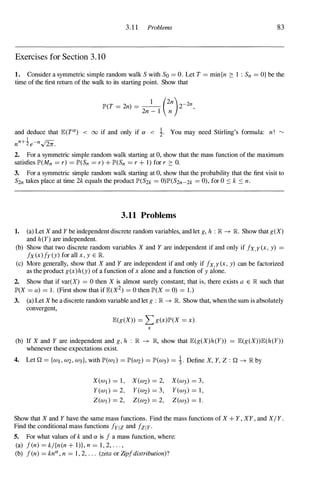
![88 3. 1 1 Discrete random variables
37. Berkson's fallacy. Any individual in a group G contracts a certain disease C with probability
y; such individuals are hospitalized with probability c. Independently of this, anyone in G may be
in hospital with probability a, for some other reason. Let X be the number in hospital, and Y the
number in hospital who have C (including those with C admitted for any other reason). Show that the
correlation between X and Y is
p(X, Y) =
where p = a + c - ac.
yp (l - a) (1 - yc)
It has been stated erroneously that, when p(X, Y) is near unity, this is evidence for a causal
relation between being in G and contracting C.
38. A telephone sales company attempts repeatedly to sell new kitchens to each of the N families
in a village. Family i agrees to buy a new kitchen after it has been solicited K; times, where the K;
are independent identically distributed random variables with mass function f(n) = IP'(K; = n). The
value 00 is allowed, so that f(oo) :::: O. Let Xn be the number of kitchens sold at the nth round of
solicitations, so that Xn = 2:�1 I{Ki=n}. Suppose that N is a random variable with the Poisson
distribution with parameter v.
(a) Show that the Xn are independent random variables, Xr having the Poisson distribution with
parameter vf(r).
(b) The company loses heart after the Tth round of calls, where T = inf{n : Xn = OJ. Let
S = XI + X2 + . . . + XT be the number of solicitations made up to time T. Show further that
JE(S) = vJE(F(T» where F(k) = f(l) + f(2) + . . . + f(k).
39. A particle performs a random walk on the non-negative integers as follows. When at the point n
(> 0) its next position is uniformly distributed on the set {O, 1, 2, . . . , n + 1}. When it hits 0 for the
first time, it is absorbed. Suppose it starts at the point a.
(a) Find the probability that its position never exceeds a, and prove that, with probability 1, it is
absorbed ultimately.
(b) Find the probability that the final step of the walk is from 1 to 0 when a = 1.
(c) Find the expected number of steps taken before absorption when a = 1.
40. Let G be a finite graph with neither loops nor multiple edges, and write dv for the degree of
the vertex v . An independent set is a set of vertices no pair of which is joined by an edge. Let
a(G) be the size of the largest independent set of G. Use the probabilistic method to show that
a(G) :::: 2:v 1/(dv + 1). [This conclusion is sometimes referred to as Turtin's theorem.]](https://image.slidesharecdn.com/grimmettstirzaker-probabilityandrandomprocessesthirded2001-220507085451-bb31ac14/85/Grimmett-Stirzaker-Probability-and-Random-Processes-Third-Ed-2001-pdf-99-320.jpg)
![90 4.1 Continuous random variables
(3) Example (2.3.4) revisited. The random variables Xand Y have density functions
{ (2n)-1
fx(x) =
0
if O s x s 2n ,
otherwise,
{ y-!/(4n) if 0S y S 4n2,
fy(y) = .
o otherWIse.
•
These density functions are non-zero if and only if x E [0,2n] and y E [0,4n2]. In such
cases in the future, we shall write simply fx(x) = (2n)-1 for O S x S 2n,and similarly for
fy,with the implicit implication that the functions in question equal zero elsewhere.
Continuous variables contrast starkly with discrete variables in that they satisfy JP>(X =
x) = 0 for all x E JR; this may seem paradoxical since X necessarily takes some value.
Very roughly speaking, the resolution of this paradox lies in the observation that there are
uncountablymany possible values for X; this number is so large that the probability of X
taking any particular value cannot exceed zero.
The numerical value f(x)is nota probability. However, we can think of f(x)dx as the
element of probability JP>(x < X S x+ dx),since
JP>(x < X s x+ dx) = F(x+ dx) -F(x) :::::: f(x)dx.
From equation (1),the probability that Xtakes a value in the interval [a,b]is
JP>(a S X S b) = lbf(x)dx.
Intuitively speaking, in order to calculate this probability, we simply add up all the small
elements of probability which contribute. More generally, if B is a sufficiently nice subset of
JR (such as an interval, or a countable union of intervals, and so on), then it is reasonable to
expect that
(4) JP>(X E B) = Inf(x)dx,
and indeed this turns out to be the case.
We have deliberately used the same letter f for mass functions and density functionst
since these functions perform exactly analogous tasks for the appropriate classes of random
variables. In many cases proofs ofresults fordiscrete variables can berewrittenforcontinuous
variables by replacing any summation sign by an integral sign, and any probability mass f(x)
by the corresponding element of probability f(x)dx.
(5) Lemma. IfXhasdensityfunctionfthen
(a) f�
oo f(x)dx = 1,
(b) JP>(X = x) = Oforallx E JR,
(c) JP>(a S X S b) = f: f(x)dx.
Proof. Exercise. •
tSome writers prefer to use the letter p to denote a mass function, the better to distinguish mass functions
from density functions.](https://image.slidesharecdn.com/grimmettstirzaker-probabilityandrandomprocessesthirded2001-220507085451-bb31ac14/85/Grimmett-Stirzaker-Probability-and-Random-Processes-Third-Ed-2001-pdf-101-320.jpg)
![4.2 Independence 91
Part (a) of the lemma characterizes those non-negative integrable functions which are
density functions of some random variable.
We conclude this section with a technical note forthe more critical reader. For what sets B
is (4) meaningful, and why does (Sa) characterize density functions? Let 'if. be the collection
of all open intervals in R By the discussion in Section 1 .6, 'if. can be extended to a unique
smallest a-field :E =a('if.) which contains 'if.; :E is called the Borel a-field and contains Borel
sets. Equation (4) holds for all B E :E. Setting IP'x (B) =IP'(X E B), we can check that
(JR, :E, IP'x) is a probability space. Secondly, suppose that f : JR -+ [0, (0) is integrable and
J�
oo f(x) dx =1 . For any B E :E, we define
IP'(B) =Inf(x) dx.
Then (JR, :E, IP') is a probability space and f is the density function of the identity random
variable X : JR -+ JR given by X (x) =x for any x E R Assiduous readers will verify the
steps of this argumentfor their own satisfaction (or see Clarke 1975, p. 53).
Exercises for Section 4. 1
1. For what values of the parameters are the following functions probability density functions?
1
(a) f(x) = C{x(l - x)}-:Z, 0 < x < 1, the density function of the 'arc sine law'.
(b) f(x) = C exp(-x - e-X), x E JR, the density function of the 'extreme-value distribution' .
(c) f(x) = C(l + x2)-m, x E R
2. Find the density function of Y = aX, where a > 0, in terms of the density function of X. Show
that the continuous random variables X and -X have the same distribution function if and only if
fx(x) = fx(-x) for all x E R
3. If f and g are density functions of random variables X and Y, show that af + (l - a)g is a
density function for 0 :5 a :5 I , and describe a random variable of which it is the density function.
4. Survival. Let X be a positive random variable with density function f and distribution function
F. Define the hazardfunction H(x) = - log[1 - F(x)] and the hazard rate
Show that:
. 1
r(x) = hm -JP'(X :5 x + h I X > x),
h,!.O h
(a) r(x) = H'(x) = f(x)/{l - F(x)},
(b) If r(x) increases with x then H(x)/x increases with x,
x � o.
(c) H(x)/x increases with x if and only if [l - F(x)]O! :5 1 - F(ax) for all 0 :5 a :5 1,
(d) If H(x)/x increases with x, then H(x + y) � H(x) + H(y) for all x, y � o.
4.2 Independence
This section contains the counterpart of Section 3.2 for continuous variables, though it con
tains a definition and theorem which hold for any pair of variables, regardless of their types
(continuous, discrete, and so on). We cannot continue to define the independence of X and Y
in terms of events such as {X =x} and {Y =y}, since these events have zero probability and
are trivially independent.](https://image.slidesharecdn.com/grimmettstirzaker-probabilityandrandomprocessesthirded2001-220507085451-bb31ac14/85/Grimmett-Stirzaker-Probability-and-Random-Processes-Third-Ed-2001-pdf-102-320.jpg)
![92 4.2 Continuous random variables
(1) DefinItion. Random variables X and Y are called independent if
(2) {X :$ x} and {Y :$ y} are independent events for all x. y E ]i.
Thereadershould verify that discrete variables satisfy (2) ifand only iftheyareindependent
in the sense of Section 3.2. Definition (1) is the general definition of the independence ofany
two variables X and Y, regardless of their types. The following general result holds for the
independence of functions of random variables. Let X and Y be random variables, and let
g, h : JR � R Then g(X) and heY) are functions which map Q into JR by
g(X)(w) = g(X (w», h(Y)(w) = h(Y(w»
as in Theorem (3.2.3). Let us suppose that g(X) and heY) are random variables. (This holds
if they are :F-measurable; it is valid for instance if g and h are sufficiently smooth or regular
by being, say, continuous or monotonic. The correct condition on g and h is actually that, for
all Borel subsets B of JR, g-I (B) and h-I (B) are Borel sets also.) In the rest of this book,
we assume that any expression oftheform 'g(X) ', where g is afunction and X is a random
variable, is itselfa random variable.
(3) Theorem. IfX and Y are independent, then so are g(X) and h(Y).
Move immediately to the next section unless you want to prove this.
Proof. Some readers may liketo try andprove this on their second reading. The proofdoes not
rely on any property such as continuity. The key lies in the requirement of Definition (2. 1 .3)
that random variables be :F-measurable, and in the observation that g(X) is :F-measurable if
g : JR � JR is Borel measurable, which is to say that g-I (B) E :13 , the Borel a-field, for all
B E :13 . Complete the proof yourself (exercise). •
Exercises for Section 4.2
1. I am selling my house, and have decided to accept the first offer exceeding £K. Assuming
that offers are independent random variables with common distribution function F, find the expected
number of offers received before I sell the house.
2. Let X and Y be independent random variables with common distribution function F and density
function f. Show that V = max{X, Y} has distribution function lP'(V .::: x) = F(x)2 and density
function fv(x) = 2f(x)F(x), x E R Find the density function of U = min{X, Y}.
3. The annual rainfall figures in Bandrika are independent identically distributed continuous random
variables {Xr : r 2: I }. Find the probability that:
(a) XI < X2 < X3 < X4,
(b) XI > X2 < X3 < X4·
4. Let {Xr : r 2: I } be independent and identically distributed with distribution function F satisfying
F(y) < 1 for all y, and let Y(y) = min{k : Xk > y}. Show that
lim lP'(Y(y) .::: lE.Y(y») = 1 - e-I.
y---+oo](https://image.slidesharecdn.com/grimmettstirzaker-probabilityandrandomprocessesthirded2001-220507085451-bb31ac14/85/Grimmett-Stirzaker-Probability-and-Random-Processes-Third-Ed-2001-pdf-103-320.jpg)
![4.3 Expectation 93
4.3 Expectation
The expectation of a discrete variable X is lEX =LxxlP'(X =x). This is an average of the
possible values of X, each value being weighted by its probability. For continuous variables,
expectations are defined as integrals.
(1) Definition. The expectation of a continuous random variable X with density function f
is given by
lEX = i:xf(x) dx
whenever this integral exists.
There are various ways of defining the integral of a function g : JR -+ JR, but it is not
appropriate to explore this here. Note that usually we shall allow the existence of J g(x) dx
only if J Ig(x)1 dx < 00.
(2) Examples (2.3.4) and (4.1.3) revisited. The random variables X and Y ofthese examples
have mean values
i2rr X
lE(X) = -dx =Jr,
o 2Jr •
Roughly speaking, the expectation operator lE has the same properties for continuous vari
ables as it has for discrete variables.
(3) Theorem. IfX and g(X) are continuous random variables then
E(g(X» = f:g(x)fx(x) dx.
We give a simple proof for the case when g takes only non-negative values, and we leave
it to the reader to extend this to the general case. Our proof is a corollary of the next lemma.
(4)Lemma. IfX has densityfunction f with f(x) =0whenx < 0,anddistributionfunction
F, then
lEX = 1
00
[1 - F(x)] dx.
Proof. [00
[1 _F(x)] dx = [00
lP'(X > x) dx = [00 [00
f(y) dy dx.
10 10 10
1y=x
Now change the order of integration in the last term.
Proof of (3) when g ::::: O. By (4),
lE(g(X» =1
00
lP'(g(X) > x) dx = 1
00
(Isfx(y) dY)dx
where B = {y : g(y) > x}. We interchange the order ofintegration here to obtain
[00 [g(y) [00
lE(g(X» =10 10
dx fx(y) dy =10
g(y)fx(y) dy.
•
•](https://image.slidesharecdn.com/grimmettstirzaker-probabilityandrandomprocessesthirded2001-220507085451-bb31ac14/85/Grimmett-Stirzaker-Probability-and-Random-Processes-Third-Ed-2001-pdf-104-320.jpg)
![94 4.3 Continuous random variables
(5) Example (2) continued. Lemma (4) enables us to find E(Y) without calculating fy, for
•
We were careful to describe many characteristics of discrete variables-such as moments,
covariance, correlation, and linearity ofE (see Sections 3.3 and 3.6)-in terms ofthe operator
E itself. Exactly analogous discussion holds for continuous variables. We do not spell out
the details here but only indicate some of the less obvious emendations required to establish
these results. For example, Definition (3.3.5) defines the kth moment of the discrete variable
X to be
(6)
we define the kth moment of a continuous variable X by the same equation. Of course, the
moments of X may not exist since the integral
may not converge (see Example (4.4.7) for an instance of this).
Exercises for Section 4.3
1. For what values of a is E(IXIO!) finite, if the density function of X is:
(a) f(x) = e-x for x 2: 0,
(b) f(x) = CO + x2)-m for x E lR?
If a is not integral, then E(IXIO!) is called the fractional moment of order a of X, whenever the
expectation is well defined; see Exercise (3.3.5).
2. Let Xl, X2, . . . , Xn be independent identically distributed random variables for which E(X;-l)
exists. Show that, if m :'0 n, then E(SmISn) = min, where Sm = Xl + X2 + . . . + Xm.
3. Let X be a non-negative random variable with density function f. Show that
for any r 2: 1 for which the expectation is finite.
4. Show that the mean /-L, median m, and variance CT2 of the continuous random variable X satisfy
(/-L - m)2 :'0 CT2.
S. Let X be a random variable with mean /-L and continuous distribution function F. Show that
if and only if a = /-L.
fa F(x) dx = roo [1 - F(x)] dx,
-00 Ja](https://image.slidesharecdn.com/grimmettstirzaker-probabilityandrandomprocessesthirded2001-220507085451-bb31ac14/85/Grimmett-Stirzaker-Probability-and-Random-Processes-Third-Ed-2001-pdf-105-320.jpg)
![4.4 Examples ofcontinuous variables
4.4 Examples of continuous variables
95
(1) Uniform distribution. The random variable X is uniform on [a, b] if it has distribution
function
{0
x - a
F(x) = t- a
if x � a ,
ifa < x � b,
if x > b.
Roughly speaking, X takes any value between a and b with equal probability. Example (2.3.4)
describes a uniform variable X. •
(2) Exponential distribution. The random variable X is exponential with parameter 'A (> 0)
if it has distribution function
(3) x 2: o.
This arises as the 'continuous limit' of the waiting time distribution of Example (3.5.5) and
very often occurs in practice as a description of the time elapsing between unpredictable
events (such as telephone calls, earthquakes, emissions of radioactive particles, and arrivals
of buses, girls, and so on). Suppose, as in Example (3.5.5), that a sequence of Bernoulli trials
is performed at time epochs 8, 28, 38, . . . and let W be the waiting time for the first success.
Then
JP'(W > k8) =(1 _ p)k and lEW =8/p.
Now fix a time t. By this time, roughly k=t/8 trials have been made. We shall let 8 -I- O. In
order that the limiting distribution lim8tO JP'(W > t) be non-trivial, we shall need to assume
that p -I- 0 also and that p/8 approaches some positive constant 'A. Then
JP'(W > t) =JP' (W > (�)8) � (1 - /..8)t/8 �e-At
which yields (3).
The exponential distribution (3) has mean
100 1
lEX = [1 - F(x)] dx =- .
o 'A
Further properties ofthe exponential distribution will be discussed in Section 4.7 and Problem
(4.1 1 .5); this distribution proves to be the cornerstone of the theory of Markov processes in
continuous time, to be discussed later. •
(4) Normal distribution. Arguably the most important continuous distribution is the normalt
(or Gaussian) distribution, which has two parameters 11 and a2and density function
1 ( X-I1)2)
f(x) = r;:;;--;)exp - 2 '
v2na2 2a
-00 < x < 00.
tProbably first named 'normal' by Francis Galton before 1 885, though some attribute the name to c. S .
Peirce, who is famous for his erroneous remark "Probability is the only branch of mathematics in which good
mathematicians frequently get results which are entirely wrong".](https://image.slidesharecdn.com/grimmettstirzaker-probabilityandrandomprocessesthirded2001-220507085451-bb31ac14/85/Grimmett-Stirzaker-Probability-and-Random-Processes-Third-Ed-2001-pdf-106-320.jpg)
![4.4 Examples ofcontinuous variables 97
If t = 1 then X is exponentially distributed with parameter A. We remark that if A = �,
t = �d, for some integer d, then X i s said to have the chi-squared distribution X2(d)with d
degrees of freedom (see Problem (4.11.12» . •
(7) Cauchy distribution. The random variable Xhas the Cauchy distributiont ifit has density
function
1
f(x) =
n(1+ x2)' -00 < x < 00.
This distribution is notable for having no moments and for its frequent appearances in counter
examples (but see Problem (4.11.4» . •
(8) Beta distribution. The random variable X is beta, parameters a, b > 0,if it has density
function
1
f(x) = __ xa-1(I _x)b-l,
B(a, b)
We denote this distribution by f3(a, b). The 'beta function'
is chosen so that f has total integral equal to one. You may care to prove that B(a, b) =
r(a)r(b)/r(a + b). If a = b = 1then X is uniform on [0,1]. •
(9) Weibull distribution. The random variable X is Weibull, parameters a,f3 > 0, if it has
distribution function
F(x) = 1 -exp(-axf x 2: 0.
Differentiate to find that
f(x) = af3xfJ-1exp(-axfJ), x 2: 0.
Set f3 = 1to obtain the exponential distribution. •
Exercises for Section 4.4
1. Prove that the gamma function satisfies r(t) = (t - l)r(t - 1) for t > 1, and deduce that
r(n) = (n - I)! for n = 1, 2, . . . . Show that r(�) = .,fii and deduce a closed form for r(n + !)
for n = 0, 1, 2, . . . .
2. Show, as claimed in (4.4.8), that the beta function satisfies B(a, b) = r(a)r(b)/ r(a + b).
3. Let X have the uniform distribution on [0, 1]. For what function g does Y = g(X) have the
exponential distribution with parameter 1?
4. Find the distribution function of a random variable X with the Cauchy distribution. For what
values of a does I X I have a finite (possibly fractional) moment of order a?
5. Log-normal distribution. Let Y = eX where X has the N(O, 1) distribution. Find the density
function of Y.
tThis distribution was considered first by Poisson, and the name is another example of Stigler's law of
eponymy.](https://image.slidesharecdn.com/grimmettstirzaker-probabilityandrandomprocessesthirded2001-220507085451-bb31ac14/85/Grimmett-Stirzaker-Probability-and-Random-Processes-Third-Ed-2001-pdf-108-320.jpg)
![98 4.5 Continuous random variables
6. Let X be N(/-t, 0"2). Show that JB:{(X - /-t)g(X») = 0"2JB:(g'(X» when both sides exist.
7. With the terminology of Exercise (4.1.4), find the hazard rate when:
(a) X has the Weibull distribution, JP'(X > x) = exp(-ax,B-l), x :::: 0,
(b) X has the exponential distribution with parameter A,
(c) X has density function af + (1 - a)g, where 0 < a < 1 and f and g are the densities of
exponential variables with respective parameters A and /-t. What happens to this last hazard rate
r(x) in the limit as x --+ oo?
8. Mills's ratio. For the standard normal density ¢(x), show that ¢'(x) + x¢(x) = O. Hence show
that
1 1 1 - <1> (x) 1 1 3
- - - < ----'---'-- < - - - + -
x x3 ¢(x) x x3 x5 '
4.5 Dependence
x > O.
Many interesting probabilistic statements about a pair X, Y of variables concern the way X
and Y vary together as functions on the same domain Q.
(1) Definition. The joint distribution function of X and Y is the function F : JR2 -+ [0, 1]
given by
F(x, y) = P(X s x , Y s y).
If X and Y are continuous then we cannot talk of their joint mass function (see Definition
(3.6.2» since this is identically zero. Instead we need another density function.
(2) Definition. The random variables X and Y are (jointly) continuous with joint (proba
biUty) density function f : JR2 -+ [0, (0) if
F(x, y) =
1:-001:-00f(u, v) du du for each x, y E JR.
If F is sufficiently differentiable at the point (x, y), then we usually specify
a2
f(x, y) = --F(x, y).
axay
The properties ofjoint distribution and density functions are very much the same as those of
the corresponding functions of a single variable, and the reader is left to find them. We note
the following facts. Let X and Y havejoint distribution function F and joint density function
f. (Sometimes we write Fx,y and fx,y to stress the roles of X and Y.)
(3) Probabilities.
JP'(a S X S b, c S Y S d) = F(b, d) - F(a, d) - F(b, c) + F(a, c)
=
i:cl�af(x, y) dx dy.](https://image.slidesharecdn.com/grimmettstirzaker-probabilityandrandomprocessesthirded2001-220507085451-bb31ac14/85/Grimmett-Stirzaker-Probability-and-Random-Processes-Third-Ed-2001-pdf-109-320.jpg)
![100 4.5 Continuous random variables
whenever F is differentiable at (x, y) (see Problem (4.14.6) also) where I, lx, Iy are taken
to be the appropriate derivatives of F, Fx and Fy .
(8) Example. Buffon's needle. A plane is ruled by the lines y = n (n = 0, ±1, ±2, . . . ) and
a needle ofunitlength is castrandomly on to the plane. What is the probability that it intersects
some line? We suppose that the needle shows no preference for position or direction.
Solution. Let (X, Y) be the coordinates of the centre of the needle and let 8 be the angle,
modulo Jr , made by the needle and the x-axis. Denote the distance from the needle's centre
and the nearest line beneath it by Z = Y - LYJ , where LYJ is the greatest integer not greater
than Y. We need to interpret the statement 'a needle is castrandomly' , and do this by assuming
that:
(a) Z is uniformly distributed on [0, 1], so that fz(z) = 1 if ° :s z :s 1 ,
(b) 8 is uniformly distributed on [0, Jr], so that le(e) = 1/Jr if O :s e :s Jr ,
(c) Z and 8 are independent, so that fz,e(z,e) = Iz (z)le(e).
Thus the pair Z, 8 has joint density function I(z,e) = 1IJr for ° :s z :s 1 , ° :s e :s Jr . Draw
a diagram to see that an intersection occurs ifand only if (Z, 8) E B where B S; [0, 1] x [0, Jr]
is given by
B = {(z,e) : Z :s !sin eor 1 -z :s !sin e}.
Hence
lh
1 in (i!Sine /1 ) 2
lP'(intersection) = I(z,e)dzde = - dz+ dz de = - .
B Jr 0 0 I-!sine Jr
Buffont designed the experiment in order to estimate the numerical value of Jr . Try it if you
have time. •
(9) Example. Bivariate normal distribution. Let I : ]R2 -+ ]R be given by
(10) I(x, y) = �exp (- 1
2 (x2 - 2pxy + y2))
2Jr 1 - p2 2(1 - p )
where p is a constant satisfying - 1 < p < 1 . Check that I is a joint density function by
verifying that
I(x, y) ::: 0, i:i:I(x, y) dx dy = 1 ;
I is called the standardbivariatenormaldensity function ofsomepair Xand Y . Calculation ot
its marginals shows that X and Y are N(O, 1) variables (exercise). Furthermore, the covariance
cov(X, Y) = JE(XY) - JE(X)JE(Y)
is given by
cov(X, Y) = i:i:xyl(x, y) dx dy = p;
tGeorges LeClerc, Comte de Buffon. In 1 777 he investigated the St Petersburg problem by flipping a coil
2084 times, perhaps the first recorded example of a Monte Carlo method in use.](https://image.slidesharecdn.com/grimmettstirzaker-probabilityandrandomprocessesthirded2001-220507085451-bb31ac14/85/Grimmett-Stirzaker-Probability-and-Random-Processes-Third-Ed-2001-pdf-111-320.jpg)
![4.5 Dependence 101
you should checkthis. Rememberthatindependentvariables are uncorrelated, butthe converse
is not true in general. In this case, however, if p = 0 then
and so X and Y are independent. We reach the following important conclusion. Standard
bivariate normal variables are independent ifand only ifthey are uncorrelated.
The general bivariate normal distribution is more complicated. We say thatthe pair X, Y has
the bivariate normal distribution with means ILl and IL2, variances at and a}, and correlation
p if theirjoint density function is
f(x, y) = �exp[- !Q(X
' Y)]
bra1a2 1 - p2
where a1 , a2 > 0 and Q is the following quadratic form
Q(x, y) =
1
[(X
-
ILI )2
_2p (�) (y
-
IL2 )+ (y
-
IL2 )2
].
(1
-
p2) al al a2 a2
Routine integrations (exercise) show that:
(a) X is N(IL1 , at) and Y is N(IL2, a}),
(b) the correlation between X and Y is p,
(c) X and Y are independent ifand only ifp = O.
Finally, here is a hint about calculating integrals associated with normal density functions.
It is an analytical exercise (Problem (4. 1 1 . 1» to show that
and hence that
1 1 2
f(x) = __ e-2X
.j2ii
is indeed a density function. Similarly, a change of variables in the integral shows that the
more general function
1
[ 1
(X - IL
)2
]
f(x) = -- exp - - --
a.j2ii 2 a
is itself a density function. This knowledge can often be used to shorten calculations. For
example, let X and Y have joint density function given by (10). By completing the square in
the exponent of the integrand, we see that
cov(X, Y) = ffxyf(x, y) dx dy
= fy �e-!Y2 (fxg(x, Y) dX)dy](https://image.slidesharecdn.com/grimmettstirzaker-probabilityandrandomprocessesthirded2001-220507085451-bb31ac14/85/Grimmett-Stirzaker-Probability-and-Random-Processes-Third-Ed-2001-pdf-112-320.jpg)
![4.5 Dependence 103
Show that fQ is a continuous joint density function whose first marginal density function is discon
tinuous at the points in Q. Can you construct a continuous joint density function whose first marginal
density function is continuous nowhere?
2. Buffon's needle revisited. Two grids of parallel lines are superimposed: the first grid contains
lines distance a apart, and the second contains lines distance b apart which are perpendicular to those
of the first set. A needle of length r « min{a, b}) is dropped at random. Show that the probability it
intersects a line equals r(2a + 2b - r)/(rrab).
3. Buffon's cross. The plane is ruled by the lines y = n, for n = 0, ±1, . . . , and on to this plane
we drop a cross formed by welding together two unit needles perpendicularly at their midpoints. Let
Z be the number of intersections of the cross with the grid of parallel lines. Show that JB:(Z/2) = 2/rr
and that
3 - ../2 4
var(Z/2) = -- - 2 .
rr rr
If you had the choice of using either a needle of unit length, or the cross, in estimating 2/rr, which
would you use?
4. Let X and Y be independent random variables each having the uniform distribution on [0, 1]. Let
U = min{X, Y} and V = max{X, Y}. Find JB:(U), and hence calculate cov(U, V).
5. Let X and f be independent continuous random variables. Show that
JB: (g(X)h (Y») = JB:(g(X»JB:(h (Y» ,
whenever these expectations exist. If X and f have the exponential distribution with parameter 1, find
JB:{exp(�(X + f» } .
6. Three points A, B, C are chosen independently at random on the circumference of a circle. Let
b(x) be the probability that at least one of the angles of the triangle ABC exceeds xrr. Show that
{ I- (3x - 1)2
b(x) =
3(1 - x)2
Hence find the density and expectation of the largest angle in the triangle.
7. Let {Xr : 1 ::s r ::s n} be independent and identically distributed with finite variance, and define
X = n-1 2:�=1 Xr . Show that cov(X, Xr - X) = o.
8. Let X and f be independent random variables with finite variances, and let U = X + Y and
V = Xf. Under what condition are U and V uncorrelated?
9. Let X and f be independent continuous random variables, and let U be independent of X and f
taking the values ±1 with probability �. Define S = UX and T = Uf. Show that S and T are in
general dependent, but S2 and T2 are independent.](https://image.slidesharecdn.com/grimmettstirzaker-probabilityandrandomprocessesthirded2001-220507085451-bb31ac14/85/Grimmett-Stirzaker-Probability-and-Random-Processes-Third-Ed-2001-pdf-114-320.jpg)
![4.6 Conditional distributions and conditional expectation 105
which is to say that Xis uniformly distributed on [0, 1]and, conditional on the event {X =x},
Y is uniform on [0,x]. In order to calculate probabilities such as lP'(X2+y2 S 1 I X =x),
say, we proceed as follows. Ifx > 0,define
A(x) = {y E � : ° S Y Sx, x2+y2 S I};
clearly A(x) = [0,minIx, .Jl - x2}]. Also,
lP'(X2+y2 S 1 I X=x) = ( jYlx (y l x)dy
lA(x)
= � min{x,Jl - x2} =min{1 , Jx-2- t }.
X
Next, let us calculate lP'(X2+y2 S 1). Let A = {(x,y) : ° S Y S x S 1, x2+y2 S I }.
Then
(4) lP'(X2+y2 S 1) =Iiix,y(x,y)dxdy
= t jx (x) ( jYIX (Y I x)dydx
lx=o lYEA(x)
=101min{l , Jx-2- I } dx =log(1 +..(2). •
From Definitions (1)and (2) it is easy to see that the conditionalexpectationof Y given X
can be defined as in Section 3.7 by lE(Y I X) =1{!(X) where
1{!(x) =lE(Y I X =x) =i:yjYlx (Y Ix)dy;
once again, lE(Y I X)has the following important property
(5) Theorem. The conditional expectation 1/t(X) = E(Y I X) satisfies
E(1/t(X) = E(Y).
We shall use this result repeatedly; it is normally written as lE(lE(Y I X») =lE(Y), and it
provides a useful method for calculating lE(Y) since it asserts that
lE(Y) =i:lE(Y I X =x)jx(x)dx.
The proof of (5) proceeds exactly as for discrete variables (see Theorem (3.7.4» ; indeed the
theorem holds for all pairs of random variables, regardless of their types. For example, in
the special case when Xis continuous and Y is the discrete random variable IB , the indicator
function of an event B,the theorem asserts that
(6) lP'(B) =lE(1{!(X» =i:lP'(B I X =x)jx(x)dx,](https://image.slidesharecdn.com/grimmettstirzaker-probabilityandrandomprocessesthirded2001-220507085451-bb31ac14/85/Grimmett-Stirzaker-Probability-and-Random-Processes-Third-Ed-2001-pdf-116-320.jpg)
![4.7 Functions ofrandom variables 107
4. Find the conditional density function and expectation of Y given X when they have joint density
function:
(a) f(x, y) = )..2e-J..y for O ::s: x ::s: y < 00,
(b) f(x, y) = xe-x(y+l) for x, y :::: o.
5. Let Y be distributed as bin(n, X), where X is a random variable having a beta distribution on
[0, } ] with parameters a and b. Describe the distribution of Y, and find its mean and variance. What
is the distribution of Y in the special case when X is uniform?
6. Let {Xr : r :::: I } be independent and uniformly distributed on [0, 1]. Let 0 < x < 1 and define
N = min{n :::: 1 : XI + X2+ . . . + Xn > x}.
Show that P(N > n) = xnIn!, and hence find the mean and variance of N.
7. Let X and Y be random variables with correlation p. Show that JE(var(Y I X)) ::s: (1 - p2) var Y.
8. Let X, Y, Z be independent and exponential random variables with respective parameters ).. , /1-, v .
Find P(X < Y < Z).
9. Let X and Y have the joint density f(x, y) = cx(y - x)e-y, O ::s: x ::s: y < 00.
(a) Find c.
(b) Show that:
fxlY(x I y) = 6x(y - x)y-3,
fylX(y I x) = (y - x)ex-y,
O ::s: x ::s: y,
O ::s: x ::s: y < 00.
(c) Deduce that JE(X I Y) = iY and JE(Y I X) = X + 2.
10. Let {Xr : r :::: O} be independent and identically distributed random variables with density
function f and distribution function F. Let N = min{n :::: 1 : Xn > Xo} and M = min{n :::: 1 :
Xo :::: XI :::: . . . :::: Xn-I < Xn }. Show that XN has distribution function F + (l - F) loge} - F),
and find P(M = m).
4.7 Functions of random variables
Let Xbe a random variable with density function I, and let g : IR � IR be a sufficiently nice
function (in the sense of the discussion after Theorem (4.2.3» . Then y = g(X)is a random
variable also. In order to calculate the distribution of Y,we proceed thust:
lP'(Y � y) = lP'(g(X) � y) = lP'(g(X) E (-00, yJ)
= lP'(X E g-I(-00, yJ) = ( I(x) dx.
Jg-l(-OO,y]
Example (2.3.4) contains an instance of this calculation, when g(x) = x2.
(1) Example. Let Xbe N(O, 1) and let g(x) = x2. Then Y = g(X) = X2 has distribution
function
lP'(Y � y) = lP'(X2 � y) = lP'(-� � X � �)
= <I>(�) - <I>(-�) = 2<1>(�)- 1 if y � 0,
tIf A � lR then g- 1 A = {x E lR : g(x ) E A}.](https://image.slidesharecdn.com/grimmettstirzaker-probabilityandrandomprocessesthirded2001-220507085451-bb31ac14/85/Grimmett-Stirzaker-Probability-and-Random-Processes-Third-Ed-2001-pdf-118-320.jpg)
![4.7 Functions a/random variables 1 1 1
Therefore, conditional on S = s, the random variable X is uniformly distributed on [0, s].
This result, and its later generalization, is ofgreat interest to statisticians. •
(9) Example. A warning. Let Xl and X2 be independent exponential variables (as in Ex
amples (7) and (8» . What is the conditional density function of Xl + X2 given Xl = X2?
'Solution' 1. Let YI = Xl + X2 and Y2 = XJ/X2. Now Xl = X2 if and only if Y2 = 1.
We have from (7) that YI and Y2 are independent, and it follows that the conditional density
function of YI is its marginal density function
(10)
'Solution' 2.
!Yl, Y3(YI, Y3)
Let YI = Xl + X2 and Y3 = XI - X2. It is an exercise to show that
�A2e-AYl for IY31 S YI, and therefore the conditional density function
of YI given Y3 is
!Y1 IY3 (YI I Y3) = Ae-A(Yl-IY31) for IY31 S YI ·
Now XI = X2 ifand only if Y3 = 0, and the required conditional density function is therefore
(11)
Something is wrong: (10) and (1 1) are different. The error derives from the original ques
tion: what does it mean to condition on the event {XI = X2}, an eventhaving probability O?
As we have seen, theanswer dependsuponhow we do the conditioning-onecannot condition
on such events quite so blithely as one may on events having strictly positive probability. In
Solution 1, we are essentially conditioning on the event {XI S X2 S (1 + h)Xd for small h,
whereas in Solution 2 we are conditioning on {XI S X2 S XI + h}; these two events contain
different sets of information. •
(12) Example. Bivariate normal distribution. Let X and Y be independent random vari
ables each having the normal distribution wth mean 0 and variance 1. Define
(13)
(14)
U = aIX,
V = a2pX + a2Hy.
where ai , a2 > 0 and Ipi < 1 . By Corollary (4), the pair U, V has joint density function
(15)
where
Q(u, v) =
1
[(�)2
_ 2p (�) (�)+ (�)2
].
(1 - p2) al al a2 a2
We deduce that the pair U, V has a bivariate normal distribution.
This factmay be used to derivemanyproperties ofthe bivariate normal distribution without
having recourse to unpleasant integrations. For example, we have that](https://image.slidesharecdn.com/grimmettstirzaker-probabilityandrandomprocessesthirded2001-220507085451-bb31ac14/85/Grimmett-Stirzaker-Probability-and-Random-Processes-Third-Ed-2001-pdf-122-320.jpg)
![1 12 4.7 Continuous random variables
whence the correlation coefficient of Uand V equals p.
Here is a second example. Conditional on the event {U = u}, we have that
Hence JE(V I U) = (o-zp/O'I)U,and var(V I U) = O'iO _ p2). •
Thetechnology above is satisfactory when thechange ofvariables is one-one,butaproblem
can arise if the transformation is many-one. The simplest examples arise of course for one
dimensional transformations. For example, if y = x2 then the associated transformation
T : x � x2 is not one-one, since it loses the sign ofx. It is easy to deal with this complication
fortransformations which are piecewise one-one (and sufficiently smooth). For example, the
above transformation T maps (-00, 0) smoothly onto (0, 00) and similarly for [0, 00): there
are two contributions tothe density function ofY = X2, one fromeach oftheintervals (-00, 0)
and [0, 00). Arguing similarly but more generally, one arrives at the following conclusion, the
proofof which is left as an exercise.
Let It , h . . . , In be intervals which partition IR (it is not important whether or not these
intervals contain their endpoints), and suppose that Y = g(x) where g is strictly monotone
and continuously differentiable on every Ii . For each i, the function g : Ii -+ IR is invertible
on g(Ii ), and we write hi for the inverse function. Then
n
(16) fY (y) = Lfx (hi (y» lh; (y) 1
i=l
with the convention that the ith summand is ° if hi is not defined at y. There is a natural
extension of this formula to transformations in two and more dimensions.
Exercises for Section 4.7
1. Let X, Y, and Z be independent and unifonnly distributed on [0, 1]. Find thejoint density function
of XY and Z2, and show that JP'(XY < Z2) = �.
2. Let X and Y be independent exponential random variables with parameter 1. Find thejoint density
function of U = X + Y and V = X/eX + y), and deduce that V is unifonnly distributed on [0, 1].
3. Let X be uniformly distributed on [0, 1n]. Find the density function of Y = sin X.
4. Find the density function of Y = sin- l
X when:
(a) X is unifonnly distributed on [0, 1],
(b) X is unifonnly distributed on [- 1, 1].
5. Let X and Y have the bivariate normal density function
f(x, y) = nexp {- 1
2 (x2 - 2pxy + i)}.
2n 1 - p2 2(1 - P )
Show that X and Z = (Y - pX)/ y'i:7 are independent N(0, 1) variables, and deduce that
1 1
JP'(X > 0, Y > 0) = - + - sin- I
p.
4 2n](https://image.slidesharecdn.com/grimmettstirzaker-probabilityandrandomprocessesthirded2001-220507085451-bb31ac14/85/Grimmett-Stirzaker-Probability-and-Random-Processes-Third-Ed-2001-pdf-123-320.jpg)
![4.8 Sums a/random variables 1 13
6. Let X and Y have the standard bivariate normal density function of Exercise (5), and define
Z = max{X, Y}. Show that E(Z) = .J(l - p)/rr, and E(Z2) = 1.
7. Let X and Y be independent exponential random variables with parameters A and /-t . Show that
Z = minIX, Y} is independent of the event {X < Y}. Find:
(a) IP'(X = Z),
(b) the distributions of U = max{X - Y, O}, denoted (X - Y)+, and V = max{X, Y} - minIX, Y},
(c) IP'(X ::::: t < X + Y) where t > O.
8. A point (X, Y) is picked at random uniformly in the unit circle. Find thejoint density of R and
X, where R2 = X2 + y2
.
9. A point (X, Y, Z) is picked uniformly at random inside the unit ball of ]R.
3
. Find the joint density
of Z and R, where R2 = X2 + y2 + Z2.
10. Let X and Y be independent and exponentially distributed with parameters A and /-t. Find the
joint distribution of S = X + Y and R = XI(X + Y). What is the density of R?
11. Find the density of Y = al(l + X2), where X has the Cauchy distribution.
12. Let (X, Y) have the bivariate normal density of Exercise (5) with 0 ::::: p < 1. Show that
pcp(b)[l - <l>(d)]
[l - <l>(a)][l - <l>(e)] ::::: IP'(X > a, Y > b) ::::: [l - <l>(a)][l - <l>(e)] +
cp(a) ,
where e = (b - pa)I �, d = (a - pb)I �, and cp and <l> are the density and distribution
function of the N(O, 1) distribution.
13. Let X have the Cauchy distribution. Show that Y = X- I
has the Cauchy distribution also. Find
another non-trivial distribution with this property of invariance.
14. Let X and Y be independent and gamma distributed as r CA , ex), r CA , fJ) respectively. Show that
W = X+ Y and Z = XI(X+ Y) are independent, and that Z has the beta distribution with parameters
ex, fJ.
4.8 Sums of random variables
This section contains an important result which is a very simple application ofthe change of
variable technique.
(1) Theorem. IfX and Y havejointdensityfunction f then X + Y has densityfunction
fx+Y (z) = i:f(x, z - x) dx.
Proof. Let A = {(x, y) : x + y S z}. Then
by the substitution x = U, Y = v + u . Reverse the order ofintegration to obtain the result. •](https://image.slidesharecdn.com/grimmettstirzaker-probabilityandrandomprocessesthirded2001-220507085451-bb31ac14/85/Grimmett-Stirzaker-Probability-and-Random-Processes-Third-Ed-2001-pdf-124-320.jpg)
![1 14 4.8 Continuous random variables
If X and Y are independent, the result becomes
fx+y(z) = L:/x(x)fy(Z - x) dx = L:/x(z - !)fy(y)dy.
The function fx+y is called the convolution of fx and fy, and is written
(2) fx+Y = fx * fy·
(3) Example. Let X and Y be independent N(O, 1) variables. Then Z = X + Y has density
function
by the substitution v = (x - �z).J2. Therefore,
showing that Z is N(O, 2) . More generally, ifX is N(J-Ll , at) and Y is N(J-L2 , ai), and X and
Y are independent, then Z = X + Y is N(J-L l + J-L2 , at+ ai) . You should check this. •
(4) Example (4.6.3) revisited. You must take great care in applying (1) when the domain of
f depends on x and y . For example, in the notation ofExample (4.6.3),
fx+Y (z) = f � dx,
A X O s z S 2,
where A = {x : 0 S z - x S x S 1} = [�z, rnin{z, 1}]. Thus
{ log 2 0 S z S 1,
fx+Y (z) =
log(2/z) 1 s z S 2.
•
(5) Example. Bivariate normal distribution. It is required to calculate the distribution of
the linear combination Z = aU'+ b V' where the pair U', V' has the bivariatenormaldensity
function of equation (4.7.15). Let X and Y be independent random variables, each having
the normal distribution with mean 0 and variance 1, and let V and V be given by equations
(4.7. 13) and (4.7. 14). It follows from the result of that example that the pairs (V, V) and
(V', V') have the samejoint distribution. Therefore Z has the same distribution as a V + bV,
which equals (aal + ba2P)X + ba2Y�. The distributionofthe last sum is easily found
by the method of Example (3) to be N(O, a
2
at+ 2abala2P + b
2
ai) . •](https://image.slidesharecdn.com/grimmettstirzaker-probabilityandrandomprocessesthirded2001-220507085451-bb31ac14/85/Grimmett-Stirzaker-Probability-and-Random-Processes-Third-Ed-2001-pdf-125-320.jpg)
![4.9 Multivariate normal distribution 1 15
Exercises for Section 4.8
1. Let X and Y be independent variables having the exponential distribution with parameters A and
/1- respectively. Find the density function of X + Y.
2. Let X and Y be independent variables with the Cauchy distribution. Find the density function of
aX + {3Y where a{3 I=- O. (Do you know about contour integration?)
3. Find the density function of Z = X + Y when X and Y have joint density function f (x, y) =
!(x + y)e-(X+Y), x, y � O.
4. Hypoexponential distribution. Let {Xr : r � I } be independent exponential random variables
with respective parameters {Ar : r � I } no two of which are equal. Find the density function of
Sn= I:�=lXr. [Hint: Use induction.]
5. (a) Let X, Y, Z be independent and uniformly distributed on [0, 1]. Find the density function of
X + Y + Z.
(b) If {Xr : r � I } are independent and uniformly distributed on [0, 1], show that the density of
I:�=I Xr at any point x E (0, n) is a polynomial in x of degree n - 1 .
6. For independent identically distributed random variables X and Y, show that U = X + Y and
V = X - Y are uncorrelated but not necessarily independent. Show that U and V are independent if
X and Y are N(O, 1).
7. Let X and Y have a bivariate normal density with zero means, variances a2, 1'2, and correlation
p. Show that:
(a) JE.(X I y) =
pa
Y,
l'
(b) var(X I y) = a2(1 - p2),
(a2 + pa1')Z
(c) JE.(X I X + Y = z) = 2 2 '
a + 2pa1' + l'
a21'2(1 _
p2)
(d) var(X I X + Y = z) =
2 2 ·
l' + 2pa1' + a
8. Let X and Y be independent N(O, 1) random variables, and let Z = X + Y. Find the distribution
and density of Z given that X > 0 and Y > O. Show that
JE.(Z I X > 0, Y > 0) = 2J2/lr.
4.9 Multivariate normal distribution
The centerpiece ofthe normal density function is the function exp(_x2), and ofthe bivariate
normal density function the function exp(_x2 - bxy - y2) for suitable b. Both cases feature
a quadratic in the exponent, and there is a natural generalization to functions of n variables
which is of great value in statistics. Roughly speaking, we say that XI , X2,...,Xnhave the
multivariate normal distribution if their joint density function is obtained by 'rescaling' the
function exp(- Lixl - 2 LkjbijXiXj)ofthe n real variables Xl,X2,...,Xn. The exponent
hereis a 'quadraticform', butnotall quadraticforms giverise to density function. A quadratic
form is a function Q : lRn -+ lRofthe form
(1) Q(x) = L aijXiXj = xAx'
l:'Oi,j:'On](https://image.slidesharecdn.com/grimmettstirzaker-probabilityandrandomprocessesthirded2001-220507085451-bb31ac14/85/Grimmett-Stirzaker-Probability-and-Random-Processes-Third-Ed-2001-pdf-126-320.jpg)
![4.9 Multivariate normal distribution 1 17
(-Xl , . . . , -Xn) are identically distributed random vectors; however, E I Xi i < 00 and so
E(Xi ) = E(-Xi ), giving E(Xi ) = O. The vector X is said to have the multivariate normal
distribution with zero means. More generally, if Y= (Yl , Y2, . . . , Yn) is given by
for some vector p, = (It] , 1t2, . . . , Itn ) of constants, then Yis said to have the multivariate
normal distribution.
(4) Definition. ThevectorX = (XI, X2 , . . . , Xn ) has themultivariate normal distribution
(or multinormal distribution), written N(p" V), if its joint density function is
where V is a positive definite symmetric matrix.
We have replaced A by V-I in this definition. The reason for this lies in part (b) of the
following theorem.
(5) Theorem. IfX is N(p" V) then
(a) lE(X) = p" which is to say that lE(Xi ) = Iti for all i,
(b) V = (Vi} ) is called the covariance matrix, because Vi} = COV(Xi , X} ).
Proof. Part (a) follows by the argument before (4). Part (b) may be proved by performing
an elementary integration, and more elegantly by the forthcoming method of characteristic
functions; see Example (5.8.6). •
We often write
V = lE«X - p,)'(X - p,))
since (X - p,)'(X - p,) is a matrix with (i, j)th entry (Xi - lti ) (X) - It} ) .
A very importantpropertyofthis distribution is its invarianceoftype under linear changes
ofvariables.
(6) Theorem. [
fX = (Xl , X2 , . . . , Xn ) is N(O, V) and Y = (YI , Y2, . . . , Ym) is given by
Y= XDfor some matrix D ofrankm S n, then Yis N(0, D'VD).
Proof when m = n. The mapping T : x t-+
y = xD is a non-singular and can be inverted as
T-I : y t-+ X = yD-i . Use this change of variables in Theorem (4.7.3) to show that, if A,
B S; ]Rn and B = T(A), then
JP>(Y E B) = f f(x) dx = r 1
exp(- �xV-Ix') dx
A fA .J(2n)nlVl
- ex _ 1 W-I , d
1 1
-
B J(2n)nIWI
p( 2Y y ) Y
where W = D'VD as required. The proof for values of m strictly smaller than n is more
difficult and is omitted (but see Kingman and Taylor 1966, p. 372). •
A similar result holds for linear transformations of N(p" V) variables.](https://image.slidesharecdn.com/grimmettstirzaker-probabilityandrandomprocessesthirded2001-220507085451-bb31ac14/85/Grimmett-Stirzaker-Probability-and-Random-Processes-Third-Ed-2001-pdf-128-320.jpg)
![4.10 Distributions arisingfrom the normal distribution
We may observe that a is only a scaling factorfor X and S(= -vfs2). That is to say,
U =
n- 1
S2 is x2(n- 1)
0'2
which does not depend on a , and
./ii -
V = -(X - J-L) IS N(O, 1)
a
which does not depend on a . Hence the random variable
V
T =
I
JTi'
Ul
Ti
(n
=
-
�
I)
121
has a distribution which does not depend on a . The random variable T is the ratio of two
independent random variables, the numerator being N(O, 1) and the denominator the square
root of (n- 1)-1 times a x2(n- 1) variable; T is said to have the tdistributionwith n - 1
degrees of freedom, written ten - 1). It is sometimes called 'Student's t distribution' in
honour of a famous experimenter at the Guinness factory in Dublin. Let us calculate its
density function. Thejoint density of U and Vis
(l)r - .! u '!r-l 1
z
e 2 u2 I 2
feu, v) = . --exp(- zv )
r(!r) 5
where r = n- 1. Then map (u,v) to (s,t) by s = u,t = v.J"i7U. Use Corollary (4.7.4) to
obtain
fU,T(S,t) = af(s,ta)
and integrate over sto obtain
r(!(r+ 1)) ( t2)-!(r+l)
fret) = I 1 + - ,
y0rTr(zr) r
as the density function of the t(r)distribution.
-00 < t < 00,
Another important distribution in statistics is the F distribution which arises as follows.
Let U and Vbe independent variables with the x2(r) and X 2(s) distributions respectively.
Then
F = Ulr
Vis
is said to have the F distribution with r and s degrees of freedom, written F(r, s). The
following properties are obvious:
(a) F-1 is F(s, r),
(b) T2is F(1, r)if T is t(r).
As an exerciseinthe techniquesofSection4.7, show thatthe density functionofthe F(r, s)
distribution is
rr(!(r+ s)) (rxls)!r-l
f�) = .
l '
sr(!r)r(!s) [1 + (rxls)]2(r+s) x > O.
In Exercises (5.7.7, 8) we shall encounter more general forms ofthe X 2,t,and F distribu
tions; these are the (so-called) 'non-central' versions ofthese distributions.](https://image.slidesharecdn.com/grimmettstirzaker-probabilityandrandomprocessesthirded2001-220507085451-bb31ac14/85/Grimmett-Stirzaker-Probability-and-Random-Processes-Third-Ed-2001-pdf-132-320.jpg)
![122 4.1 1 Continuous random variables
Exercises for Section 4. 1 0
1. Let XI and X2 be independent variables with the X
2(m) and X
2(n) distributions respectively.
Show that Xl + X2 has the x
2(m + n) distribution.
2. Show that the mean of the t(r) distribution is 0, and that the mean of the F(r, s) distribution is
s/(s - 2) if s > 2. What happens if s ::::: 2?
3. Show that the t(l) distribution and the Cauchy distribution are the same.
4. Let X and Y be independentvariables having theexponential distribution with parameter 1. Show
that XI Y has an F distribution. Which?
5. Use the result of Exercise (4.5.7) to show the independence of the sample mean and sample
variance of an independent sample from the N(f,L, 0"2) distribution.
6. Let {Xr : 1 ::::: r ::::: n} be independent N(O, 1) variables. Let IJI E [0, Jr] be the angle
between the vector (XI , X2, . . . , Xn) and some fixed vector in ]R.n. Show that IJI has density
1(1/1) = (sin 1/I)n-2IB(i, in - !), 0 ::::: 1/1 < Jr , where B is the beta function.
4.11 Sampling from a distribution
It is frequently necessary to conduct numerical experiments involving random variables with
a given distributiont. Such experiments are useful in a wide variety of settings, ranging from
the evaluation of integrals (see Section 2.6) to the statistical theory of image reconstruction.
The target of the current section is to describe a portfolio of techniques for sampling from
a given distribution. The range of available techniques has grown enormously over recent
years, and we give no more than an introduction here. The fundamentalquestion is as follows.
Let F be a distribution function. How may we find a numerical value for a random variable
having distribution function F?
Various interesting questions arise. What does it mean to say that a real numberhas a non
trivial distribution function? In auniverse whose fundamentalrulesmaybe deterministic, how
can one simulate randomness? In practice, one makes use of deterministic sequences ofreal
numbersproducedby whatare called 'congruentialgenerators'. Such sequences are sprinkled
uniformly over their domain, and statistical tests indicate acceptance of the hypothesis that
they are independent and uniformly distributed. Strictly speaking, these numbers are called
'pseudo-random' but the prefix is often omitted. They are commonly produced by a suitable
computer program called a 'random number generator'. With a little cleverness, such a
program may be used to generate a sequence UI , U2, . . . of(pseudo-)random numbers which
may be assumed to be independentanduniformly distributedon the interval [0, 1]. Henceforth
in this section we will denote by U a random variable with this distribution.
A basic way of generating a random variable with given distribution function is to use the
following theorem.
(1) Theorem. Inverse transform technique. Let F be a distributionfunction, and let U be
uniformly distributed on the interval [0, 1].
(a) If F is a continuous junction, the random variable X = F-1 (U) has distribution
junction F.
tSuch experiments are sometimes referred to as 'simulations' .](https://image.slidesharecdn.com/grimmettstirzaker-probabilityandrandomprocessesthirded2001-220507085451-bb31ac14/85/Grimmett-Stirzaker-Probability-and-Random-Processes-Third-Ed-2001-pdf-133-320.jpg)
![4.1 1 Samplingfrom a distribution 123
(b) Let F be the distribution function of a random variable taking non-negative integer
values. The random variable X given by
X = k ifand only if F(k - 1) < U .:s F(k)
hasdistributionfunction F.
Proof. Part (a) is Problem (4.14.4a). Part (b) is a straightforward exercise, on noting that
lP'(F(k - 1) < U .:s F(k») = F(k) - F(k - 1).
This part of the theorem is easily extended to more general discrete distributions. •
The inverse transform technique is conceptually easy but has practical drawbacks. In
the continuous case, it is required to know or calculate the inverse function F-1 ; in the
discrete case, a large number ofcomparisons may be necessary. Despite the speed ofmodem
computers, such issues remain problematic forextensive simulations.
Here are three examples of the inverse transform technique in practice. Further examples
may be found in the exercises at the end ofthis section.
(2)Example. Binomialsampling. Let Ul, U2, . . . , Un, . . . beindependentrandomvariables
with the uniform distribution on [0, 1]. The sequence Xk = I{uk:'!:.p) of indicator variables
contains random variables having the Bernoulli distribution with parameter p. The sum
S = L�=1 Xk has the bin(n, p) distribution. •
(3) Example. Negative binomial sampling. With the Xk as in the previous example, let Wr
be given by
Wr = min{n : tXk = r },
k=l
the 'time of the rth success'. Then Wr has the negative binomial distribution; see Example
(3.5.6). •
(4) Example. Gamma sampling. With the Uk as in Example (2), let
It is an easy calculation (or use Problem (4.14.4a» to see that the Xk are independent expo
nential random variables with parameter A.. It follows that S = L�=l Xk has the r(A., n)
distribution; see Problem (4. 14.10). •
Here are two further methods of sampling from a given distribution.
(5) Example. The rejection method. It is required to sample from the distribution having
densityfunction f. Letus suppose that we areprovidedwithapair (U, Z) ofrandomvariables
such that:
(i) U and Z are independent,
(ii) U is uniformly distribution on [0, 1], and
(iii) Z has density function fz, and there exists a E lR such that f(z) .:s afz(z) for all z .](https://image.slidesharecdn.com/grimmettstirzaker-probabilityandrandomprocessesthirded2001-220507085451-bb31ac14/85/Grimmett-Stirzaker-Probability-and-Random-Processes-Third-Ed-2001-pdf-134-320.jpg)
![124 4.1 1 Continuous random variables
We note the following calculation:
Now,
f�oo P(aUfz(Z) :s feZ)IZ=z)fz(z)dz
p(z < x I aUfz(Z) < feZ)) = .
- -
f�
oo P(aUfz(Z) :s feZ) I Z=z)fz(z)dz
I
fez)
P(aUfz(Z) :s feZ) Z=z) =p(u :s f(z)/{afz(z)l) = -
afz(z)
whence
p(Z :SxIaUfz(Z) :s feZ)) =i�f(z)dz.
That is to say, conditional on the event E = {aUfz(Z) :s feZ)},the random variable Zhas
the required density function f.
We use this fact in the following way. Let us assume that one may use a random number
generator to obtain a pair (U, Z)as above. We then check whether or not the event Eoccurs.
If Eoccurs, then Zhas the required density function. If Edoes not occur, we rejectthe pair
(U, Z),and use the random number generatorto find another pair (U', Z/)with the properties
(i)-(iii) above. This process is iterated until the event corresponding to E occurs, and this
results in a sample from the given density function.
Each sample pair (U, Z) satisfies the condition of Ewith probability a. It follows by the
independence ofrepeated sampling thatthe mean numberofsamples before Eis first satisfied
is a-I.
A similar technique exists for sampling from a discrete distribution. •
(6) Example. Ratio of uniforms. There are other 'rejection methods' than that described in
the above example, and here is a further example. Once again, let f be a density function
from which a sample is required. For a reason which will become clear soon, we shall assume
that f satisfies f(x) = ° if x :s 0, and f(x) :s min{1, x-2}if x > 0. The latter inequality
may be relaxed in the following, but at the expense of a complication.
Suppose that UI and U2 are independent and uniform on [0, 1], and define R = U2/UI.
We claim that, conditional on the event E = {UI :s .Jf(U2/UI)}, the random variable R
has density function f. This provides the basis for a rejection method using uniform random
variables only. We argue as follows in order to show the claim. We have that
where T = {(UI,U2) : UI .:s .Jf(U2/UJ), U2 .:s xut}. We make the change of variables
s =U2/UI,t =UI,to obtain that
r
[nw
r
p(En{R :Sx}) =Js=o Jt=o
tdtdS= !Jo f(s)ds,
from which it follows as required that
P(R :s x I E) = lax f(s)ds. •](https://image.slidesharecdn.com/grimmettstirzaker-probabilityandrandomprocessesthirded2001-220507085451-bb31ac14/85/Grimmett-Stirzaker-Probability-and-Random-Processes-Third-Ed-2001-pdf-135-320.jpg)
![4.1 1 Samplingfrom a distribution 125
In samplingfromadistributionfunction F, the structure ofF may itselfpropose a workable
approach.
(7) Example. Mixtures. Let Fl and F2 be distribution functions and let ° .:s a .:s 1. It is
required to sample from the 'mixed' distribution function G = aFt + (1 - a)F2. This may
be done in a process of two stages:
(i) first toss a coin which comes up heads with probability a (or, more precisely, utilize the
random variable I(U:,,:a) where U has the usual uniform distribution),
(ii) if the coin shows heads (respectively, tails) sample from Ft (respectively, F2)'
As an example ofthis approach in action, consider the density function
1
g(x) = "-----,, + 3x(1 - x),
Jr'l 1 - x2
and refer to Theorem (1) and Exercises (4.1 1.5) and (4.l 1.13). •
This example leads naturally to the following more general formulation. Assume that the
distribution function G may be expressed in the form
G(x) = lE(F(x, Y», x E JR,
where Y is a random variable, and where F(·, y) is a distribution function for each possible
value y of Y. Then G may be sampled by:
(i) sampling from the distribution of Y, obtaining the value y, say,
(ii) sampling from the distribution function F(·, y).
(8) Example. Compound distributions. Here is a further illustrative example. Let Z have
the beta distribution with parameters a and b, and let
k = 0, 1, 2, . . . , n.
It is an exercise to show that
Pk ex: G)r(a + k)r(n + b - k), k = 0, 1, 2, .. . , n,
where r denotes the gamma function; this distribution is termed a negative hypergeometric
distribution. In sampling from the mass function (Pk : k = 0, 1, 2, . . . , n) it is convenient to
sample firstfromthe beta distribution of Z and then from the binomial distribution bin(n, Z);
see Exercise (4.1 1.4) and Example (2). •
Exercises for Section 4. 1 1
1. Uniform distribution. If U is uniformly distributed on [0, 1], what is the distribution of X =
LnUJ + l?
2. Random permutation. Given the first n integers in any sequence So, proceed thus:
(a) pick any position Po from {l, 2, . . . , n} at random, and swap the integer in that place of So with
the integer in the nth place of So, yielding St.](https://image.slidesharecdn.com/grimmettstirzaker-probabilityandrandomprocessesthirded2001-220507085451-bb31ac14/85/Grimmett-Stirzaker-Probability-and-Random-Processes-Third-Ed-2001-pdf-136-320.jpg)
![126 4.1 1 Continuous random variables
(b) pick any position PI from { I , 2, . . . , n - I } at random, and swap the integer in that place of S1
with the integer in the (n - I)th place of SI, yielding S2,
(c) at the (r - I)th stage the integer in position Pr-l, chosen randomly from { I , 2, . . . , n - r + I },
is swapped with the integer at the (n - r + I)th place of the sequence Sr-l.
Show that Sn-l is equally likely to be any of the n! permutations of { l , 2, . . . , n}.
3. Gammadistribution. Use the rejection method to sample from the gamma density r(A , t) where
t (� 1) may not be assumed integral. [Hint: You might want to start with an exponential random
variable with parameter l it.]
4. Beta distribution. Show how to sample from the beta density f3(a, f3) where a, f3 � 1. [Hint:
Use Exercise (3).]
5. Describe three distinct methods of sampling from the density f(x) = 6x( l - x), 0 :::: x :::: 1 .
6. Aliasing method. A finite real vector is called a probability vector if it has non-negative entries
with sum 1 . Show that a probability vector p of length n may be written in the form
1
n
P = - L Vr,
n - 1
r=1
where each Vr is a probability vector with at most two non-zero entries. Describe a method, based on
this observation, for sampling from p viewed as a probability mass function.
7. Box-Muller normals. Let UI and U2 be independent and uniformly distributed on [0, 1 ], and
let Ti = 2Ui - 1 . Show that, conditional on the event that R = VTl + Ti :::: 1 ,
X = �V-2 10g R2, y = ;V-2 10g R2 ,
are independent standard normal random variables.
8. Let U be uniform on [0, 1] and 0 < q < 1. Show that X = 1 + Llog UIlog qJ has a geometric
distribution.
9. A point (X, Y) is picked uniformly at random in the semicircle x2 + i :::: 1 , x � O. What is the
distribution of Z = YI X?
10. Hazard-rate technique. Let X be a non-negative integer-valued random variable with her) =
JP'(X = r I X � r). If {Ui : i � O} are independent and uniform on [0, 1], show that Z = min{n :
Un :::: hen)) has the same distribution as X.
11. Antithetic variables. Let g(Xl , X2 , . . . , xn) be an increasing function in all its variables, and
let fUr : r � l } be independent and identically distributed random variables having the uniform
distribution on [0, 1]. Show that
[Hint: Use the FKG inequality of Problem (3. 10. 1 8).] Explain how this can help in the efficient
estimation of I = JJ g(x) dx.
12. Importance sampling. We wish to estimate I = J g(x)fx(x) dx = JE(g(X)), where either it
is difficult to sample from the density fx, or g(X) has a very large variance. Let fy be equivalent
to fx, which is to say that, for all x, fx(x) = 0 if and only if fy(x) = O. Let {Yi : 0 :::: i :::: n} be
independent random variables with density function fy, and define](https://image.slidesharecdn.com/grimmettstirzaker-probabilityandrandomprocessesthirded2001-220507085451-bb31ac14/85/Grimmett-Stirzaker-Probability-and-Random-Processes-Third-Ed-2001-pdf-137-320.jpg)
![Show that:
4.12 Coupling and Poisson approximation
(a) II':(J) = [ = II': [g(y)fx(Y)]
fy(Y) ,
(b) var(J) = � [II': (g(Y)2fx(Y)2) _ [2],
n fy(Y)2
(c) J � [ as n ---+ 00. (See Chapter 7 for an account of convergence.)
127
The idea here is that fyshould be easy to sample from, and chosen if possible so that var J is
much smaller than n-1[II':(g(X)2) - [2]. The function fyis called the importance density.
13. Construct two distinct methods of sampling from the arc sin density
2
f(x)= � '
Ji V 1 - x-
4.12 Coupling and Poisson approximation
It is frequently necessary to compare the distributions of two random variables X and Y.
Since X and Y may not be defined on the same sample space Q, it is in general impossible
to compare X and Y themselves. An extremely useful and modem technique is to construct
copies X' and yl (of X and Y) on the same sample space Q, and then to compare X' and yl.
This approach is known as couplingt, and it has many important applications. There is more
than one possible coupling of a pair X and Y, and the secret of success in coupling is to find
the coupling which is well suited to the particular application.
Note thatanytwo distributions may be coupled in a trivial way, since one may always find
independent random variables X and Y with the required distributions; this may be done via
the constructionofaproductspaceas in Section 1.6. This couplinghas little interest, precisely
because the value of X does not influence the value of y.
(1) Example. Stochastic ordering. Let X and Y be random variables whose distribution
functions satisfy
(2) Fx(x) ::::: Fy(x) for all x E lR.
In this case, we say that X dominates Y stochastically and we write X 2:st y. Note that X
and Y need not be defined on the same probability space.
The following theorem asserts in effectthat X 2:st Y if and only if there exist copies of X
and Y which are 'pointwise ordered' .
(3) Theorem. Suppose that X 2:st Y. There exists a probability space (Q , F, lP') and two
random variable X' and yl on this space such that:
(a) X' and X have the same distribution,
(b) yl and Y have the same distribution,
(c) lP'(X' 2: yl) = 1.
tThe tenn 'coupling' was introduced by Frank Spitzer around 1 970. The coupling method was developed by
W. Doeblin in 1938 to study Markov chains. See Lindvall (1992) for details of the history and the mathematics
of coupling.](https://image.slidesharecdn.com/grimmettstirzaker-probabilityandrandomprocessesthirded2001-220507085451-bb31ac14/85/Grimmett-Stirzaker-Probability-and-Random-Processes-Third-Ed-2001-pdf-138-320.jpg)
![128 4.12 Continuous random variables
Proof. Take Q = [0, 1], :F the Borel a-field of Q, and let JP' be Lebesgue measure, which is
to say that, for any sub-interval I of Q, JP'(I) is defined to be the length of I.
For any distribution function F, we may define a random variable ZF on (Q , :F, JP') by
ZF(W) = inf{z : W ::::: F(z)}. W E Q .
Note that
(4) W ::::: F(z) if and only if ZF(W) ::::: z.
It follows that
JP'(ZF ::::: z) = JP'([O, F(z)1) = F(z),
whence ZF has distribution function F.
Suppose now that X :=:st Y and write G and H for the distribution functions of X and
Y. Since G(x) ::::: H(x) for all x, we have from (4) that ZH ::::: ZG. We set X' = ZG and
y' = ZH. • •
Here is a more physical coupling.
(5) Example. ButTon's weldings. Suppose we cast at random two of Buffon's needles (in
troduced in Example (4.5.8» , labelled NJ and N2. Let X (respectively, Y) be the indicator
function of a line-crossing by NJ (respectively, N2). Whatever the relationship between NJ
and N2, we have that JP'(X = 1) = JP'(Y = 1) = 2177:. The needles may however be coupled
in various ways.
(a) The needles are linked by a frictionless universaljoint at one end.
(b) The needles are welded at their ends to form a straight needle with length 2.
(c) The needles are weldedperpendicularly at their midpoints, yieldingthe Buffon cross of
Exercise (4.5.3).
We leave it as an exercise to calculate for each of these weldings (or 'couplings') the
probability that both needles intersect a line. •
(6) Poisson convergence. Consider a large number ofindependent events each having small
probability. In a sense to be made more specific, the number of such events which actually
occurhas a distribution which is close to a Poisson distribution. An instance ofthis remarkable
observation was the proofin Example (3.5.4) that the bin(n, 'Aln) distribution approaches the
Poisson distribution with parameter 'A, in the limit as n -+ 00. Here is a more general result,
proved using coupling.
Thebettertostatetheresult, weintroduce firstametriconthespaceofdistributionfunctions.
Let F and G be the distribution functions ofdiscrete distributions whichplace masses fnand
gnat the points xn, for n :=: 1, and define
(7) dTV(F, G) = LIfk -gkl·
k:o:J
The definition ofdTV(F, G) may be extendedto arbitrary distribution functions as in Problem
(7.1 1 .16); the quantity dTV(F, G) is called the total variation distancet between F and G.
tSome authors define the total variation distance to be one half of that given in (7).](https://image.slidesharecdn.com/grimmettstirzaker-probabilityandrandomprocessesthirded2001-220507085451-bb31ac14/85/Grimmett-Stirzaker-Probability-and-Random-Processes-Third-Ed-2001-pdf-139-320.jpg)
![130 4.12 Continuous random variables
(10) Example. Set Pr = )../n for 1 � r � n to obtain the inequality dTV(S, P) � 2)..2/n,
which provides a rate of convergence in the binomial-Poisson limit theorem of Example
05�. •
In many applications ofinterest, the Bernoulli trials Xrare not independent. Nevertheless
one may prove a Poisson limit theorem so long as they are not 'too dependent'. A beautiful
way of doing this is to use the so-called 'Stein-Chen method', as follows.
As before, we suppose that {Xr : 1 � r � n} are Bernoulli random variables with
respective parameters Pr,but we make no assumption concerning their independence. With
S = .E�=I Xr, we assume that there exists a sequence VI,V2,...,Vn of random variables
with the property that
(11) JP'(Vr = k- 1) = JP'(S= k I Xr = 1), 1 � k � n.
[We may assume that Pr =1= 0 for all r, whence JP'(Xr = 1) > 0.] We shall see in the
forthcoming Example (14)how such Vrmay sometimes be constructed in a natural way.
(12) Theorem. Stein-Chen approximation. Let P bea random variablehaving thePoisson
distribution with parameter ).. = .E�=I pro The total variation distance between S and P
satisfies
n
dTV(S, P) � 2(1 / )..-1 ) LPrEIS-Vrl.
r=1
Recall thatx / y = min {x,y}. The bound fordTV(X, Y) takes a simple formin a situation
where JP'(S 2: Vr) = 1for every r. If this holds,
n n n
LPrEIS- Vrl = LPr(E(S)-E(Vr») = )..2 -LPrE(Vr).
r=1 r=1 r=1
By (11),
n n
PrE(Vr) = PrL(k- 1)JP'(S= k I Xr = 1) = L(k- 1)JP'(Xr = 1 I S = k)JP'(S= k)
k=1 k=1
n
= L(k- I)E(Xr I S= k)JP'(S= k),
k=1
whence n n
r=1 k=1
It follows by Theorem (12)that, in such a situation,
(13)
Before proving Theorem (12),we give an example of its use.
(14) Example. Balls in boxes. There are m balls and n boxes. Each ball is placed in a box
chosen uniformly at random, different balls being allocated to boxes independently of one](https://image.slidesharecdn.com/grimmettstirzaker-probabilityandrandomprocessesthirded2001-220507085451-bb31ac14/85/Grimmett-Stirzaker-Probability-and-Random-Processes-Third-Ed-2001-pdf-141-320.jpg)
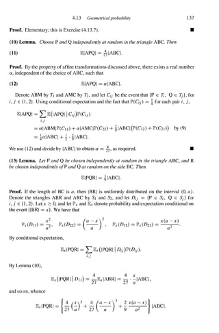
![4.13 Geometricalprobability
The circles are the shapes SI and S2 . The shaded regions are denoted A and B, and b(X) is
the sum of the perimeter lengths of A and B.
139
3. Let SI and S2 be convex figures such that S2 S; S1 . Show that the probability that two independent
random lines AI and A2, crossing S], meet within S2 is 2n IS21Ib(SI)2, where IS21 is the area of S2
and b(SI) is the length of the boundary of SI . (See Example (4.13.2) for an explanation of the term
'random line'.)
4. Let Z be the distance between two points picked independently at random in a disk of radius a.
Show that E(Z) = 128al(45n), and E(Z2) = a2.
5. Pick two points A and B independently at random in a ball with centre O. Show that the probability
that the angle AoB is obtuse is �. Compare this with the corresponding result for two points picked
at random in a circle.
6. A triangle is formed by A, B, and a point P picked at random in a set S with centre of gravity G.
Show that EIABPI = IABGI .
7. A point D is fixed on the side BC ofthe triangle ABC. Two points P and Qare picked independently
at random in ABD and ADC respectively. Show that EIAPQI = IAGI G21 = �IABC ! , where Gl and
G2 are the centres of gravity of ABD and ADC.
8. From the set of all triangles that are similar to the triangle ABC, similarly oriented, and inside
ABC, one is selected uniformly at random. Show that its mean area is toIABC! .
9. Two points X and Y are picked independently at random in the interval (0, a). By varying a,
show that F(z, a) = JP'(lX - YI :::: z) satisfies
aF 2 2z
- + -F = -,
aa a a2 0 :::: z :::: a,
and hence find F(z, a). Let r 2: 1 , and show that mr(a) = E(lX - yn satisfies
Hence find mr(a).
10. Lines are laid down independently at random on the plane, dividing it into polygons. Show that
the average number of sides of this set of polygons is 4. [Hint: Consider n random great circles of a
sphere of radius R ; then let R and n increase.]
11. A point P is picked at random in the triangle ABC. The lines AP, BP, CP, produced, meet BC,
AC, AB respectively at L, M, N. Show that EILMNI = (10 - n2) IABC ! .
12. Sylvester's problem. If four points are picked independently at random inside the triangle ABC,
show that the probability that no one of them lies inside the triangle formed by the other three is �.
13. Ifthree points P, Q,R are picked independently at random in a diskofradiusa, show that EIPQRI =
35a2/(48n). [You may find it useful that fer fer sin
3
x sin
3
y sin Ix - yl dx dy = 35n1 1 28.]](https://image.slidesharecdn.com/grimmettstirzaker-probabilityandrandomprocessesthirded2001-220507085451-bb31ac14/85/Grimmett-Stirzaker-Probability-and-Random-Processes-Third-Ed-2001-pdf-150-320.jpg)
![140 4.14 Continuous random variables
14. Two points A and B are picked independently at random inside a disk C. Show that the probability
that the circle having centre A and radius IAB l lies inside C is i.
15. Two points A and B are picked independently at random inside a ball S . Show that the probability
that the sphere having centre A and radius IAB l lies inside S is do.
4.14 Problems
1. (a) Show that J::O
oo e-x2 dx = ../ii, and deduce that
1 { (X- J-t)2}
f(x) = I'C exp -
2 '
u'V2:n: 2u
-00 < x < 00,
is a density function if u > O.
(b) Calculate the mean and variance of a standard normal variable.
(c) Show that the N(0, 1) distribution function <I> satisfies
These bounds are of interest because <I> has no closed form.
x > O.
(d) Let X be N(O, 1), and a > O. Show that IP'(X > x + a/x I X > x) -7 e-a as x -7 O.
2. Let X be continuous with density function f(x) = C(x - x2), where a < x < f3 and C > O.
(a) What are the possible values of a and f3 ?
(b) What is C?
3. Let X be a random variable which takes non-negative values only. Show that
00 00
L)i - 1)IAi .::: X < L ilAi '
i=l i=l
where Ai = {i - 1 .::: X < i}. Deduce that
00 00
L IP'(X :::: i) '::: E(X) < 1 + L IP'(X :::: i).
i=l i=1
4. (a) Let X have a continuous distribution function F. Show that
(i) F(X) is uniformly distributed on [0, 1],
(ii) - log F(X) is exponentially distributed.
(b) A straight line I touches a circle with unit diameter at the point P which is diametrically opposed
on the circle to another point Q. A straight line QRjoins Q to some point R on I. Ifthe angle PQR
between the lines PQ and QR is a random variable with the uniform distribution on [- �:n:, �:n:],
show that the length ofPR has the Cauchy distribution (this length is measured positive ornegative
depending upon which side of P the point R lies).
5. Let X have an exponential distribution. Show that IP'(X > s + x I X > s) = JP'(X > x), for
x, s :::: O. This is the 'lack of memory' property again. Show that the exponential distribution is the
only continuous distribution with this property. You may need to use the fact that the only non-negative
monotonic solutions of the functional equation g(s + t) = g(s)g(t) for s, t :::: 0, with g(O) = 1, are
of the form g(s) = elLS. Can you prove this?](https://image.slidesharecdn.com/grimmettstirzaker-probabilityandrandomprocessesthirded2001-220507085451-bb31ac14/85/Grimmett-Stirzaker-Probability-and-Random-Processes-Third-Ed-2001-pdf-151-320.jpg)
![142 4.14 Continuous random variables
17. If X and Y are independent random variables, show that U = min{X, Y } and V = max{X, Y }
have distribution functions
FU (u) = 1 - {1 - Fx(u)}{1 - Fy(u)}, Fv(v) = Fx(v)Fy(v).
Let X and Y be independent exponential variables, parameter 1 . Show that
(a) U is exponential, parameter 2,
(b) V has the same distribution as X + iY. Hence find the mean and variance of V.
18. Let X and Y be independent variables having the exponential distribution with parameters A and
/l, respectively. Let U = min{X, Y}, V = max{X, Y}, and W = V - U.
(a) Find JP'(U = X) = JP'(X :'0 Y).
(b) Show that U and W are independent.
19. Let X and Y be independent non-negative random variables with continuous density functions
on (0, (0).
(a) If, given X + Y = u, X is uniformly distributed on [0, u] whatever the value of u, show that X
and Y have the exponential distribution.
(b) If, given that X + Y = u, X/u has a given beta distribution (parameters a and fJ, say) whatever
the value of u, show that X and Y have gamma distributions.
You may need the fact that the only non-negative continuous solutions of the functional equation
g(s + t) = g(s)g(t) for s, t 2: 0, with g(O) = 1 , are of the form g(s) = elLS. Remember Problem
(4. 14.5).
20. Show that it cannot be the case that U = X + Y where U is uniformly distributed on [0, 1] and X
and Y are independent and identically distributed. You should not assume that X and Y are continuous
variables.
21. Orderstatistics. LetXI, X2, . . . , Xnbeindependentidentically distributed variables with a com
mon density function f. Such a collection is called a randomsample. Foreach W E Q, arrangethe sam
ple values XI (W), . . . , Xn(w) in non-decreasing order X(l)(w) :'0 X(2)(W) :'0 . . . :'0 X(n)(w), where
(1) , (2), . . . , (n) is a (random) permutation of 1 , 2, . . . , n. The new variables X(l), X(2), · · · , X(n)
are called the order statistics. Show, by a symmetry argument, that the joint distribution function of
the order statistics satisfies
JP'(X(l) :'0 YI, . . . , X(n) :'0 Yn) = n! JP'(XI :'0 YI , . . . , Xn :'0 Yn, Xl < X2 < . . . < Xn)
where L is given by
and x = (Xl , x2, . . . , Xn).
n! L(y)f(Yl) · · · f(Yn)·
= J. . . (I':::Yl L(XI , . . . , Xn)n! f(XI) . . . f(xn) dXI . . . dXn
J�2':::Y2
L(x) = { � if Xl < X2 < . . . < Xn,
otherwise,
Deduce that the joint density function of X(1), . . . , X(n) is g(y)
22. Find the marginal density function of the kth order statistic X(k) of a sample with size n:
(a) by integrating the result of Problem (4. 14.21),
(b) directly.
23. Find thejoint density function of the order statistics ofn independent uniform variables on [0, T).
24. Let Xl, X2, . . . , Xn be independent and uniformly distributed on [0, 1], with order statistics
XCI)' X(2), . . . , X(n)·
(a) Show that, for fixed k, the density function of nX(k) converges as n ---+ 00, and find and identify
the limit function.](https://image.slidesharecdn.com/grimmettstirzaker-probabilityandrandomprocessesthirded2001-220507085451-bb31ac14/85/Grimmett-Stirzaker-Probability-and-Random-Processes-Third-Ed-2001-pdf-153-320.jpg)
![4.14 Problems 143
(b) Show that log X(k) has the same distribution as - 'L,7=k i-I Yi, where the Yi are independent
random variables having the exponential distribution with parameter 1.
(c) Show that Zl , Z2, . . . , Zn, defined by Zk = (X(k)/X(k+l) k for k < n and Zn = (X(n) n, are
independent random variables with the uniform distribution on [0, 1].
25. Let Xl , X2, X3 be independent variables with the uniform distribution on [0, 1]. What is the
probability that rods of lengths Xb X2, and X3 may be used to make a triangle? Generalize your
answer to n rods used to form a polygon.
26. Let Xl and X2 be independent variables with the uniform distribution on [0, 1]. A stick of unit
length is broken at points distance Xl and X2 from one of the ends. What is the probability that the
three pieces may be used to make a triangle? Generalize your answer to a stick broken in n places.
27. Let X, Y be a pair ofjointly continuous variables.
(a) HOlder's inequality. Show that if p, q > 1 and p-1 + q-1 = 1 then
Set p = q = 2 to deduce the Cauchy-Schwarz inequality JB:(XY)2 :::: JB:(x2)JB:(y2).
(b) Minkowski's inequality. Show that, if p ::: 1, then
Note that in both cases your proof need not depend on the continuity of X and Y; deduce that the same
inequalities hold for discrete variables.
28. Let Z be a random variable. Choose X and Y appropriately in the Cauchy-Schwarz (or Holder)
inequality to show that g(p) = log JB:I ZP I is a convex function of p on the interval of values of p such
that JB:I ZP I < 00. Deduce Lyapunov's inequality:
You have shown in particular that, if Z has finite rth moment, then Z has finite sth moment for all
positive s :::: r.
29. Show that, using the obvious notation, JB:{JB:(X I Y, Z) I y} = JB:(X I Y).
30. Motor cars of unit length park randomly in a street in such a way that the centre of each car, in
tum, is positioned uniformly at random in the space available to it. Let m(x) be the expected number
of cars which are able to park in a street of length x. Show that
1 loX
m(x + l) = - {m(y) + m(x - y) + I } dy.
x 0
It is possible to deduce that m(x) is about as big as �x when x is large.
31. ButTon's needle revisited: ButTon's noodle.
(a) A plane is ruled by the lines y = nd (n = 0, ±1, . . . ). A needle with length L « d) is cast
randomly onto the plane. Show that the probability that the needle intersects a line is 2L/(nd).
(b) Now fix the needle and let C be a circle diameter d centred at the midpoint of the needle. Let
A be a line whose direction and distance from the centre of C are independent and uniformly
distributed on [0, 2n] and [0, 1d] respectively. This is equivalent to 'casting the ruled plane at
random' . Show that the probability of an intersection between the needle and A is 2L/(nd).
(c) Let S be a curve within C having finite length L(S). Use indicators to show that the expected
number of intersections between S and A is 2L(S)/(nd).
This type of result is used in stereology, which seeks knowledge of the contents of a cell by studying
its cross sections.](https://image.slidesharecdn.com/grimmettstirzaker-probabilityandrandomprocessesthirded2001-220507085451-bb31ac14/85/Grimmett-Stirzaker-Probability-and-Random-Processes-Third-Ed-2001-pdf-154-320.jpg)
![144 4.14 Continuous random variables
32. Buffon's needle ingested. In the excitement of calculating n, Mr Buffon (no relation) inadver
tently swallows the needle and is X-rayed. If the needle exhibits no preference for direction in the
gut, what is the distribution of the length of its image on the X-ray plate? If he swallowed Buffon's
cross (see Exercise (4.5.3» also, what would be the joint distribution of the lengths of the images of
the two arms of the cross?
33. Let XI , X2, . . . , Xn be independent exponential variables with parameter A, and let X(l) <
X(2) :::: . . . :::: X(n) be their order statistics. Show that
are also independent and have the same joint distribution as the Xi .
34. Let X(l) , X(2) , . . . , X(n) be the order statistics of a family ofindependent variables with common
continuous distribution function F. Show that
1 :::: r < n,
are independent and uniformly distributed o n [0, 1]. This i s equivalent to Problem (4. 14.33). Why?
35. Secretary/marriage problem. You are permitted to inspect the n prizes at a fete in a given order,
at each stage either rejecting or accepting the prize under consideration. There is no recall, in the sense
that no rejected prize may be accepted later. It may be assumed that, given complete information, the
prizes may be ranked in a strict order of preference, and that the order of presentation is independent
of this ranking. Find the strategy which maximizes the probability of accepting the best prize, and
describe its behaviour when n is large.
36. Fisher's spherical distribution. Let R
2
= X
2
+ y
2
+ Z
2
where X, Y, Z are independent normal
random variables with means A , j.t, v, and common variance 0-
2
, where (A, j.t, v) =I (0, 0, 0). Show
that the conditional density of the point (X, Y, Z) given R = r, when expressed in spherical polar
coordinates relative to an axis in the direction e = (A , j.t, v), is of the form
f(e, ¢» = � eacose sine, 0 :::: e < n, 0 :::: ¢> < 2n,
4n smh a
where a = riel.
37. Let ¢> be the N(O, 1 ) density function, and define the functions Hn , n :::: 0, by Ho = 1 , and
(_ l)n Hn¢> = ¢>(n) , the nth derivative of ¢>. Show that:
(a) Hn (x) is a polynomial of degree n having leading term xn , and
foo { O if m =I n,
-
00
Hm (x)Hn (x)¢> (x) dx =
n! if m = n.
00
tn
(b) '" Hn (x) - = exp(tx - 1t2
).
� n!
n=O
38. Lancaster's theorem. Let X and Y have a standard bivariate normal distribution with zero
means, unit variances, and correlation coefficient p, and suppose U = u (X) and V = v(Y) have finite
variances. Show that Ip(U, V)I :::: Ipl. [Hint: Use Problem (4. 14.37) to expand the functions u and
v. You may assume that u and v lie in the linear span of the Hn .]
39. Let X(1) , X(2) , . . . , X(n) be the order statistics of n independent random variables, uniform on
[0, 1]. Show that:
r r(n - s + l)
(a) JE(X(r) =
n + l ' (b) cov(X(r) , X(s) =
(n + 1)2 (n +
2) for r :::: s.](https://image.slidesharecdn.com/grimmettstirzaker-probabilityandrandomprocessesthirded2001-220507085451-bb31ac14/85/Grimmett-Stirzaker-Probability-and-Random-Processes-Third-Ed-2001-pdf-155-320.jpg)
![4.14 Problems 145
40. (a) Let X, Y, Z be independent N(O, 1) variables, and set R = VX2 + y2 + Z2. Show that
X2/R2 has a beta distribution with parameters ! and 1, and is independent of R2.
(b) Let X, Y, Z be independent and uniform on [- 1, 1] and set R = VX2 + y2 + Z2. Find the
density of X2/R2 given that R2 .::: 1.
41. Let c/J and <1> be the standard normal density and distribution functions. Show that:
(a) <1> (x) = 1 - <1> (-x),
(b) f(x) = 2c/J (x)<1> (AX), -00 < x < 00, is the density function of some random variable (denoted
by Y), and that IYI has density function 2c/J.
(c) LetXbea standardnormal random variableindependentofY, anddefine Z = (X+A IYI)/Vi + A2.
Write down the joint density of Z and IYI, and deduce that Z has density function f.
42. The six coordinates (Xi, Yi), 1 .::: i .::: 3, of three points A, B, C in the plane are independent
N(O, 1). Show that the the probability that C lies inside the circle with diameter AB is !.
43. The coordinates (Xi, Yi, Zi), 1 .::: i .::: 3 , of three points A, B , C are independent N(O, 1). Show
that the probability that C lies inside the sphere with diameter AB is ! _ .J3.
3 411
44. Skewness. Let X have variance 0'2 and write mk = JB:(Xk). Define the skewness of X by
skw(X) = JB:[(X - ml )3]jO'3. Show that:
(a) skw(X) = (m3 - 3mlm2 + 2mi)/O'3,
(b) skw(Sn) = skw(XI )/..jn, where Sn = 2:�=1 Xr is a sum of independent identically distributed
random variables,
(c) skw(X) = (1 - 2p)/-Jnpq, when X is bin(n, p) where p + q = 1,
(d) skw(X) = 1/...fi., when X is Poisson with parameter A,
(e) skw(X) = 2/0, when X is gamma r(A, t), and t is integral.
45. Kurtosis. Let X have variance 0'2 and JB:(Xk) = mk. Define the kurtosis of X by kur(X)
JB:[(X - ml)4]/O'4. Show that:
(a) kur(X) = 3, when X is N(I-i, 0'2),
(b) kur(X) = 9, when X is exponential with parameter A,
(c) kur(X) = 3 + A-I , when X is Poisson with parameter A,
(d) kur(Sn) = 3 + {kur(XI) - 3)jn, where Sn = 2:�=1 Xr is a sum of independent identically
distributed random variables.
46. Extreme value. Fisher-Gumbel-Tippett distribution. Let Xr, 1 .::: r .::: n, be independent and
exponentially distributed with parameter 1. Show that X(n) = max{Xr : 1 .::: r .::: n} satisfies
lim JP'(X(n) - log n .::: x) = exp(-e-X).
n-+oo
Hence show that Jooo{I - exp(_e-X)} dx = y where y is Euler's constant.
47. Squeezing. Let S and X have density functions satisfying b(x) .::: fs(x) .::: a(x) and fs (x) .:::
fx(x). Let U be uniformly distributed on [0, 1] and independent of X. Given the value X, we
implement the following algorithm:
if Ufx(X) > a(X), reject X;
otherwise: if Ufx(X) < b(X), accept X;
otherwise: if Ufx(X) .::: fs(X), accept X;
otherwise: reject X.
Show that, conditional onultimate acceptance, X is distributed as S. Explain when you mightuse this
method of sampling.](https://image.slidesharecdn.com/grimmettstirzaker-probabilityandrandomprocessesthirded2001-220507085451-bb31ac14/85/Grimmett-Stirzaker-Probability-and-Random-Processes-Third-Ed-2001-pdf-156-320.jpg)
![146 4.14 Continuous random variables
48. Let X, Y, and {Ur : r :::: I } be independent random variables, where:
x 1
IP'(X = x) = (e - l)e- , IP'(Y = y) = for x, y = 1 , 2, . . . ,
(e - l)y!
and the Ur are uniform on [0, 1]. Let M = max{UI , U2, . . . , Uy }, and show that Z = X - M is
exponentially distributed.
49. Let U and V be independent and uniform on [0, 1]. Set X = _a-l log U and Y = - log V
where a > O.
1 2
(a) Show that, conditional on the event Y :::: 1(X - a)2, X has density function f(x) = ,J2/rre-2
x
for x > O.
(b) In sampling from the density function f, it is decided to use a rejection method: for given a > 0,
we sample U and V repeatedly, and we accept X the first time that Y :::: i(X - a)2. What is the
optimal value of a?
(c) Describe how to use these facts in sampling from the N(O, 1) distribution.
50. Let S be a semicircle of unit radius on a diameter D.
(a) A point P is picked at random on D. If X is the distance from P to S along the perpendicular to
D, show IE(X) = rr/4.
(b) A point Q is picked at random on S. If Y is the perpendicular distance from Q to D, show
IE(Y) = 2/rr.
51. (Set for the Fellowship examination of St John's College, Cambridge in 1 858.) 'A large quantity
of pebbles lies scattered uniformly over a circular field; compare the labour of collecting them one by
one:
(i) at the centre 0 of the field,
(ii) at a point A on the circumference.'
To be precise, if Lo and LA are the respective labours per stone, show that IE(Lo) = �a and
IE(LA) = 32a/(9rr) for some constant a.
(iii) Suppose you take each pebble to the nearer of two points A or B at the ends of a diameter. Show
in this case that the labour per stone satisfies
4a { 16 17 1 } 2
IE(LAB) =
3rr 3" - 6.J2 + 2" log(1 + .J2) � 1. 13 x 3"a.
(iv) Finally suppose you take each pebble to the nearest vertex ofan equilateral triangle ABC inscribed
in the circle. Why is it obvious that the labour per stone now satisfies IE(LABc) < IE(Lo)?
Enthusiasts are invited to calculate IE(LABc).
52. The lines L, M, and N are parallel, and P lies on L. A line picked at random through P meets M
at Q. A line picked at random through Q meets N at R. What is the density function of the angle e
that RP makes with L? [Hint: Recall Exercise (4.8.2) and Problem (4. 14.4).]
53. Let � denote the event that you can form a triangle with three given parts of a rod R.
(a) R is broken at two points chosen independently and uniformly. Show that IP'(�) = *.
(b) R is broken in two uniformly at random, the longer part is broken in two uniformly at random.
Show that IP'(�) = log(4/e).
(c) R is broken in two uniformly at random, a randomly chosen part is broken into two equal parts.
Show that IP'(�) = i.
(d) In case (c) show that, given �, the triangle is obtuse with probability 3 - 2.J2.
54. You break a rod at random into two pieces. Let R be the ratio ofthe lengths ofthe shorter to the
longer piece. Find the density function JR, together with the mean and variance of R.
55. Let R be the distance between two points picked at random inside a square of side a. Show that](https://image.slidesharecdn.com/grimmettstirzaker-probabilityandrandomprocessesthirded2001-220507085451-bb31ac14/85/Grimmett-Stirzaker-Probability-and-Random-Processes-Third-Ed-2001-pdf-157-320.jpg)
![5
Generating functions and their applications
Summary. A key method forstudying distributions is via transforms such as the
probability generating function of a discrete random variable, or the moment
generating function and characteristic function of a general random variable.
Such transforms are particularly suited to the study of sums of independent
random variables, andtheirareasofapplicationincluderenewaltheory,random
walks, and branching processes. The inversion theorem tells how to obtain
the distribution function from knowledge of its characteristic function. The
continuity theorem allows us to use characteristic functions in studying limits
ofrandom variables. Twoprincipal applications areto thelaw oflargenumbers
and the central limit theorem. The theory of large deviations concerns the
estimation of probabilities of 'exponentially unlikely' events.
5.1 Generating functions
A sequence a = {ai : i = 0, 1, 2, . . . } ofreal numbers may contain a lot ofinformation. One
concise way of storing this information is to wrap up the numbers together in a 'generating
function'. For example, the (ordinary) generatingfunction of the sequence ais the function
Ga defined by
00
(1) Ga(s) = L aisi for s E lR for which the sum converges.
i=O
The sequence a may in principle be reconstructed from the function Ga by setting ai
G�i)(0)/i !, where f(i) denotes the ith derivative ofthe function f. In many circumstances it
is easier to work with the generating function Gathan with the original sequence a.
(2) Example. De Moivre's theorem. The sequence an = (cos B + i sin B)n has generating
function 00
1
Ga(s) = "'[s(cos B + i sin B)f = . .
� 1 - s(cos B + I sm B)
n=O
if IsI < 1; here i = A. It is easily checked by examining the coefficient ofsn that
00
[1 - s(cos B + i sin B)] Lsn [cos(nB) + i sin(nB)] = 1
n=O](https://image.slidesharecdn.com/grimmettstirzaker-probabilityandrandomprocessesthirded2001-220507085451-bb31ac14/85/Grimmett-Stirzaker-Probability-and-Random-Processes-Third-Ed-2001-pdf-159-320.jpg)
![5.1 Generatingfunctions
when lsi < 1. Thus
00 1
Lsn[cos(ne) + i sin(ne)] = . .
1 - s(cos e + 1 sm e)
n=O
149
if IsI < 1. Equating the coefficients of sn we obtain the well-known fact that cos(ne) +
i sin(ne) = (cose + i sin e)n. •
There are several differenttypes ofgenerating function,ofwhich Gaisperhaps the simplest.
Another is the exponential generatingfunction Eagiven by
(3)
00 aisi
Ea(s) = L -
.-
, for s E lR. for which the sum converges.
I .
i=O
Whilst such generating functions have many uses in mathematics, the ordinary generating
function (1 ) is ofgreater value when the ai are probabilities. This is because 'convolutions'
are common in probability theory, and (ordinary) generating functions provide an invaluable
tool for studying them.
(4) Convolution. Theconvolutionofthereal sequencesa = {ai : i ::: O} andb = {bi : i ::: O}
is the sequence c = {Ci : i ::: O} defined by
(5)
we write c = a * b. If a and bhave generating functions Ga and Gb,then the generating
function of c is
(6) Gc(s) = fcnsn = f(i>ibn-i)sn
n=O n=O i=O
00 00
= LaisiLbn_iSn-i = Ga(S)Gb(S).
i=O n=i
Thus we learn that, if c = a * b, then Gc(s) = Ga(S)Gb(S); convolutions are numerically
complicated operations, and it is often easier to work with generating functions.
(7) Example. The combinatorial identity
may be obtained as follows. The left-hand side is the convolution of the sequence ai = (7),
i = 0, 1, 2, . . . , with itself. However, Ga(s) = Li (7)si = (1 + s)n,so that
2 2n '"(2n
) i
GaM(s) = Ga(s) = (1 + s) = �
i
s .
I
Equating the coefficients ofsnyields the required identity. •](https://image.slidesharecdn.com/grimmettstirzaker-probabilityandrandomprocessesthirded2001-220507085451-bb31ac14/85/Grimmett-Stirzaker-Probability-and-Random-Processes-Third-Ed-2001-pdf-160-320.jpg)
![150 5. 1 Generatingfunctions and their applications
(8) Example. Let X and Y be independent random variables having the Poisson distribution
with parameters A and /Lrespectively. What is the distribution of Z = X + Y?
Solution. We have from equation (3.8.2) that the mass function of Z is the convolution of
the mass functions of X and Y, fz = fx * fy. The generating function of the sequence
{fx(i) : i :?: O} is
(9)
00
Ai -J..
G (s) = '"' _
e
_si = eJ..(s-I)
x � .f '
l .
i=O
and similarly Gy(s) = ell(s-l). Hence the generating function Gzof (fz(i) :i :?: O}satisfies
Gz(s) = Gx(s)Gy(s) = exp[(A +/L)(s- 1)], which we recognize from (9) asthe generating
function of the Poisson mass function with parameter A + /L. •
The last example is canonical: generating functions provide a basic technique for dealing
with sums ofindependentrandomvariables. Withthis examplein mind, wemakean important
definition. Suppose that X is a discrete random variable taking values in the non-negative
integers {O, 1, 2, . . . }; its distribution is specified by the sequence of probabilities f(i) =
JP'(X = i).
(10) DefInition. The (probability)generatingfunction of the random variable X is defined
to be the generating function G(s) = JE(sx) ofits probability mass function.
Note that Gdoes indeed generate the sequence (f(i) : i :?: O} since
by Lemma (3.3.3). We write Gx when we wish to stress the role of X. If X takes values
in the non-negative integers, its generating function Gx converges at least when IsI ::s 1 and
sometimesin alarger interval. Generating functions can be definedforrandom variablestaking
negative as well as positive integer values. Such generating functions generally converge for
values of s satisfying a < lsi < f3 for some a, f3 such that a ::s 1 ::s f3. We shall make
occasional use ofsuch generating functions, but we do notdevelop theirtheory systematically.
In advance of giving examples and applications ofthe method ofgenerating functions, we
recall some basic properties ofpower series. Let G(s) = L:g" aisi where a = {ai : i :?: O}is
a real sequence.
(11) Convergence. Thereexists a radiusofconvergence R(2: 0) such that the sumconverges
absolutely if IsI < Rand diverges if IsI > R. The sum is uniformly convergent on sets ofthe
form {s : lsi ::s R'}for any R' < R.
(12) Differentiation. Ga(s)may be differentiatedor integrated term by term any number of
times at points s satisfying lsi < R.
(13) Uniqueness. If Ga(s) = Gb(S)for lsi < R'where 0 < R' ::s Rthen an = bn for all n.
Furthermore
(14) a = �c<n)(o)
n f a ·
n.](https://image.slidesharecdn.com/grimmettstirzaker-probabilityandrandomprocessesthirded2001-220507085451-bb31ac14/85/Grimmett-Stirzaker-Probability-and-Random-Processes-Third-Ed-2001-pdf-161-320.jpg)
![5.1 Generatingfunctions 151
(15) Abel's theorem. Ifai 2: 0 for all i and Ga(s)is finite for lsi < 1,then limstl Ga(s) =
L�oai, whether the sum is finite or equals +00. This standard result is useful when the
radius ofconvergence R satisfies R = 1,since then one has no a priori right to take the limit
ass t 1.
Returning to the discrete random variable X taIdng values in {O, 1,2, . . . } we have that
G(s) = L�silP'(X = i), so that
(16) G(O) = lP'(X = 0), G(I) = 1.
In particular, the radius ofconvergence ofa probability generating function is at least 1. Here
are some examples of probability generating functions.
(17) Examples.
(a) Constant variables. 1flP'(X = c) = 1then G(s) = E(sx) = sC.
(b) Bernoulli variables. 1flP'(X = 1) = p and lP'(X= 0) = 1 -p then
G(s) = E(sx) = (1 -p) + ps.
(c) Geometric distribution. If X is geometrically distributed with parameter p, so that
lP'(X = k) = p(1 -p)k-I for k 2: 1,then
00
G(s) = E(sx) = I>kp(1 _
p)k-l =
ps
.
1 -s(1 -p)
k= l
(d) Poisson distribution. If Xis Poisson distributed with parameter A then
•
Generating functions are useful when working with integer-valued random variables. Prob
lems arise when random variables take negative or non-integer values. Later in this chapter
we shall see how to construct another function, called a 'characteristic function', which is
very closely related to Gx but which exists for all random variables regardless oftheir types.
There are two major applications of probability generating functions: in calculating mo
ments, andincalculatingthedistributions ofsumsofindependentrandomvariables. Webegin
with moments.
(18) Theorem. IfXhas generatingfunction G(s) then
(a) E(X) = G'(1),
(b) more generally, E[X(X- 1)...(X -k + 1)] = G(kl(1).
Ofcourse, G(kl(1)is shorthand for limstl G(kl(s) whenever the radius ofconvergence of G
is 1. The quantity E[X(X- 1)···(X-k + 1)]is known as the kthfactorial moment of X.
Proofof (b). Take s < 1 and calculate the kth derivative of Gto obtain
dkl(S) = I>i-ki(i - 1)···(i - k + l)f(i) = E[sX-kX(X- 1)···(X-k + 1)].
i](https://image.slidesharecdn.com/grimmettstirzaker-probabilityandrandomprocessesthirded2001-220507085451-bb31ac14/85/Grimmett-Stirzaker-Probability-and-Random-Processes-Third-Ed-2001-pdf-162-320.jpg)
![152 5.1 Generatingfunctions and their applications
Let s t 1 and use Abel's theorem (15)to obtain
G(
k) (S) -+ I>(i - 1)···(i - k + l)f(i) = JE[X(X- 1)···(X- k +1)]. •
In order to calculate the variance of Xin terms of G,we proceed as follows:
(19) var(X) = JE(X2)-JE(X)2 = JE(X(X- 1)+X) - JE(X)2
= JE(X(X- 1)) +JE(X)- JE(X)2 = G"(I)+G'(1)-G'(1)2.
Exercise. Find the means and variances ofthe distributions in (17)by this method.
(20) Example. Recall the hypergeometric distribution (3.11.10)with mass function
f(k) = G)(��:)/(�).
Then G(s) = Lkskf(k),which can be recognized as the coefficient ofxn in
Q(s,x) = (1 +sx)b(1 +x)N-b/(�).
Hence the mean G'(1)is the coefficient ofxn in
a
a�(1,x) = xb(1+x)N-l/(�)
and so G'(1) = bnjN. Now calculate the variance yourself (exercise). •
If you are more interested in the moments of Xthan in its mass function, you may prefer
to work not with Gx but with the function Mx defined by Mx(t) = Gx (et). This change of
variable is convenient for the following reason. Expanding Mx (t) as a power series in t,we
obtain
(21)
00 00 00
( k)n
Mx(t) = Letkjp'(X = k) = L L �jp'(X = k)
k=O k=On=O
theexponentialgenerating function ofthe momentsJE(Xo),JE(X1),. . . ofX. The function Mx
is called the momentgeneratingfunctionofthe random variable X. We have assumed in (21)
thatthe seriesinquestion converge. Somecomplications can ariseinusing momentgenerating
functions unless the series LntnJE(Xn)jn!has a strictly positive radius ofconvergence.
(22) Example. We have from (9) that the moment generating function of the Poisson distri
bution with parameter 'A is M(t) = exp['A (et - 1)]. •](https://image.slidesharecdn.com/grimmettstirzaker-probabilityandrandomprocessesthirded2001-220507085451-bb31ac14/85/Grimmett-Stirzaker-Probability-and-Random-Processes-Third-Ed-2001-pdf-163-320.jpg)
![5.1 Generatingfunctions 155
Exercises for Section 5 . 1
1. Find the generating functions of the following mass functions, and state where they converge.
Hence calculate their means and variances.
(a) f(m) = (
n+:-l)pn (l - p)m, for m 2: O.
(b) f(m) = {m(m + 1)}-1, for m 2: 1.
(c) f(m) = (I - p)plml /(l + p), for m = . . . , -1, 0, I, . . . .
The constant p satisfies 0 < p < I.
2. Let X (2: 0) have probability generating function G and write t(n) = JP'(X > n) for the 'tail'
probabilities of X. Show that the generating function of the sequence {t(n) : n 2: O} is T(s) =
(l - G(s» /(l - s). Show that E(X) = T(l) and var(X) = 2T'(l) + T(1) - T(1)2.
3. Let Gx,y (s, t) be the joint probability generating function of X and Y. Show that GX (s) =
Gx,Y(s, I) and Gy(t) = Gx,y (l, t). Show that
E(XY) = --Gx y(s, t) .
a2
I
as at '
s=t=1
4. Find thejoint generating functions ofthe followingjoint mass functions, and state for what values
ofthe variables the series converge.
(a) f(j, k) = (1 - a)(fJ - a)ajfJk-j-1, for O ::s k ::s j, where 0 < a < I, a < fJ.
(b) f(j, k) = (e - 1)e-(2k+l)kj/j !, for j, k 2: O.
(c) f(j, k) = (�)pj+k(l - p)k-j/[k log{I/(1 - p)}], for O ::S j ::s k, k 2: I, where 0 < p < 1.
Deduce the marginal probability generating functions and the covariances.
5. A coin is tossed n times, and heads turns up with probability p on each toss. Assuming the usual
independence, show that thejoint probability generating function of the numbers H and T of heads
and tails is GH,T(X, y) = {px + (1 - p)y}n. Generalize this conclusion to find thejoint probability
generating function ofthe multinomial distribution of Exercise (3.5.1).
6. Let X have the binomial distribution bin(n, U), where U is uniform on (0, 1). Show that X is
uniformly distributed on {O, 1, 2, . . . , n}.
7. Show that
G(X, y, z, w) = l(xyzw + xy + yz + zw + zx + yw + xz + 1)
is thejoint generating function offour variables that are pairwise and triplewise independent, but are
nevertheless not independent.
8. Let Pr > 0 and ar E � for 1 ::s r ::s n. Which ofthe following is a moment generating function,
and for what random variable?
n n
(a) M(t) = I + 2: Prtr, (b) M(t) = 2: Preart.
r=1 r=1
9. Let Gl and G2 be probability generating functions, and suppose that 0 ::s a ::s 1. Show that
G] G2, and aG] + (l - a)G2 are probability generating functions. Is G(as)/G(a) necessarily a
probability generating function?](https://image.slidesharecdn.com/grimmettstirzaker-probabilityandrandomprocessesthirded2001-220507085451-bb31ac14/85/Grimmett-Stirzaker-Probability-and-Random-Processes-Third-Ed-2001-pdf-166-320.jpg)
![5.2 Some applications 157
the first letter is put into its correct envelope, and let Nbe the event that no match occurs.
Then
(6)
where lP'(MC) = 1 - n-I . It is convenient to think of an =lP'(N I MC)in the following way.
It is the probability that, given n - 2 pairs of matching white letters and envelopes together
with a non-matchingred letter and blue envelope, there are no colour matches when the letters
are inserted randomly into the envelopes. Either the red letter is placed into the blue envelope
or it is not, and a consideration of these two cases gives that
(7) an = _
1
_Pn_2+ (1 - _
1
_)an-I.
n - I n - l
Combining (6) and (7) we obtain, for n � 3,
(8) Pn = (1 - �)an = (1 - �) [n �1
Pn-2+ (1 -
n �1 )an-I]
= (1 - �)(n �1
Pn-2+ pn-l) = �Pn-2+ (I - �)Pn-I,
a difference relation subject to the boundary conditions PI =0,P2 = �. We may solve this
difference relation by using the generating function
(9)
00
G(s) =LPnsn.
n=1
We multiply throughout (8) by nsn-I and sum over all suitable values ofn to obtain
00 00 00
" n-l " n-2 "( 1) n-2
�ns Pn =s�s Pn-2+s� n- s Pn-I
n=3 n=3 n=3
which we recognize as yielding
G'(s) - PI -2P2S =sG(s)+ s[G'(s)- ptl
or (1 -s)G'(s) =sG(s)+ s,since PI =0and P2 = �. This differential equation is easily
solved subject to the boundary condition G(O) = 0to obtain G(s) = (1 -s)-le-s - 1.
Expanding as a power series in sand comparing with (9), we arrive at the conclusion
(10)
(_l)n (_l)n-1 (-1)
Pn = -
-
, - +
( - 1) ' + · · · + -
1 ,- + 1, for n � l,
n. n . .
as in the conclusion of Example (3.4.3) with r =O. •](https://image.slidesharecdn.com/grimmettstirzaker-probabilityandrandomprocessesthirded2001-220507085451-bb31ac14/85/Grimmett-Stirzaker-Probability-and-Random-Processes-Third-Ed-2001-pdf-168-320.jpg)
![r
,
160 5.2 Generatingfunctions and their applications
Returning to (17), we obtain similarly that U(x) = L�1 x
n
Un satisfies
(21)
D(x)
U(x) = D(X)GH(X) = ---
1 - F(x)
where D(x) is the probability generating function ofXI . Equation (21) contains much ofthe
information relevant to the process, since it relates the occurrences of H to the generating
functions ofthe elements of the sequence XI , X2 , . . . . We should like to extract information
out of(21) about Un = IP'(Hn), the coefficient ofx
n
in U(x), particularly for large values ofn.
In principle, one may expand D(x)/[l - F(x)] as a polynomial in x in order to find Un,
but this is difficult in practice. There is one special situation in which this may be done with
ease, and this is the situation when D(x) is the function D = D* given by
(22) *
1 - F(x)
D (x) = for IxI < 1,
1t(1 - x)
and It = E(X2) is the mean inter-occurrence time. Let us first check that D* is indeed a
suitable probability generating function. The coefficient of xn in D* is easily seen to be
(1 - It - h- . . . - fn)/It, where fi = IP'(X2 = i). This coefficient is non-negative since
the fi form a mass function; furthermore, by L'H6pital's rule,
D*(1) = lim
1 - F(x)
= lim
_F'(X)
= 1
xtl 1t(1 - x) xtl -It
since F'(I) = It, the mean inter-occurrence time. Hence D*(x) is indeed a probability
generating function, and with this choice for D we obtain that U = U* where
(23) U*(x) =
1
1t(1 - x)
from (21). Writing U*(x) = Ln u�xn
we find that u� = It- I for all n. That is to say, for
the special choice of D*, the corresponding sequence of the u� is constant,so that the density
of occurrences of H is constant as time passes. This special process is called a stationary
recurrent-eventprocess.
Howrelevant is the choice ofD tothe behaviourofUn for large n? Intuitively speaking, the
choice of distribution of XI should not affect greatly the behaviour of the process over long
time periods, and so one mightexpectthatUn � It- I as n � 00, irrespective ofthechoice of
D. This is indeed the case, so long as we rule out the possibility that there is 'periodicity' in
the process. We call the process non-arithmeticifgcd{n : IP'(X2 = n) > O} = 1 ; certainly the
process is non-arithmetic if, for example, IP'(X2 = 1) > O. Note that gcd stands for greatest
common divisor.
(24) Renewal theorem. Ifthemeaninter-occurrencetimeIt isfiniteandtheprocessisnon
arithmetic,thenUn = IP'(Hn) satisfiesUn � It- I
asn � 00.
Sketch proof. The classical proof of this theorem is a purely analytical approach to the
equation (21) (see Feller 1968, pp. 335-8). There is a much neater probabilistic proof using
the technique of 'coupling'. We do not give a complete proof at this stage, but merely a
sketch. The main idea is to introduce a second recurrent-event process, which is stationary](https://image.slidesharecdn.com/grimmettstirzaker-probabilityandrandomprocessesthirded2001-220507085451-bb31ac14/85/Grimmett-Stirzaker-Probability-and-Random-Processes-Third-Ed-2001-pdf-171-320.jpg)
![(1) Theorem. Wehavethat:
(a) Po(s) = 1 + Po(s)Fo(s),
(b) Po(s) = (1 -4pqs2)-!,
(c) Fo(s) = 1 -(1 -4pqs2)!.
5.3 Random walk 163
Proof. (a) Let A be the event that Sn = 0, and let Bk be the event that the first return to the
origin happens at the kth step. Clearly the Bk are disjoint and so, by Lemma (1.4.4),
n
lP'(A) = LlP'(A I Bk)lP'(Bk).
k=l
However, lP'(Bk) = fo(k) and lP'(A I Bk) = po(n- k) by temporal homogeneity, giving
(2)
n
po(n) = Lpo(n- k)fo(k) if n � 1 .
k=l
Multiply (2) by sn, sum over nremembering that po(O) = 1, and use the convolutionproperty
of generating functions to obtain Po(s) = 1 + Po(s)Fo(s).
(b) Sn = 0 ifand only ifthe particle takes equal numbers ofsteps to the left and to the right
during its first nsteps. The number of ways in which it can do this is (l.n
n) and each such way
2
occurs with probability (pq)n/2,giving
(3)
We have that po(n) = 0 if nis odd. This sequence (3) has the required generating function
Po(s).
(c) This follows immediately from (a) and (b). •
(4) Corollary.
(a) Theprobabilitythattheparticleeverreturnstotheoriginis
00
Lfo(n) = Fo(1) = 1 - Ip-ql·
n=]
(b) Ifeventualreturnis certain, thatisFo(1) = 1 andp = i, thentheexpectedtimetothe
firstreturnis 00
Lnfo(n) = F�(l) = 00.
n=!
We call the process persistent (or recurrent)if eventual return to the origin is (almost)
certain; otherwise it is called transient. It is immediately obvious from (4a) thatthe process
is persistent ifandonly if p= i. This is consistent with our intuition, which suggests that if
p > i or p < i, then the particle tends to stray a long way to the right or to the left of the
origin respectively. Even when p= i the time until first return has infinite mean.](https://image.slidesharecdn.com/grimmettstirzaker-probabilityandrandomprocessesthirded2001-220507085451-bb31ac14/85/Grimmett-Stirzaker-Probability-and-Random-Processes-Third-Ed-2001-pdf-174-320.jpg)
![164 5.3 Generatingfunctions and theirapplications
Proof. (a) Let s t 1 in (lc), and remember equation (5.1.30).
(b) Eventual return is certain ifandonly if p= i. But then the generating function ofthe
time To to the first return is Fo(s) = 1 -(l -s2)! and lE(To) = limstl F�(s)= 00. •
Now let us consider the times of visits to the point r. Define
Ir(n) = lP'(SI =1= r,. . . , Sn-I =1= r, Sn = r)
to be the probability that the first such visit occurs at the nth step, with generating function
Fr(s) = L�I Ir(n)sn.
(5) Theorem. We have that:
(a) Fr(s) = [FI (s)Ylorr 2: 1,
(b) FI(s) = [1 -(1 -4pqs2)!]/(2qs).
Proof. (a) The same argument which yields (2)also shows that
n-l
Ir (n) = Llr-l (n - k)/l (k) if r > 1.
k=1
Multiply by snand sum over n to obtain
We could have written this out in terms ofrandom variables instead ofprobabilities, and then
used Theorem (5.1.23). To see this, let Tr = min{n : Sn = r}be the number of steps taken
before the particle reaches rfor the first time (Tr may equal +00 if r > 0 and p < i or if
r < 0 and p > i). In order to visit r,the particle must first visit the point 1;this requires n
steps. After visiting 1the particle requires a further number, TI,r say, of steps to reach r;TI,r
is distributed in the manner of Tr-I by 'spatial homogeneity'. Thus
if n = 00,
if TI < 00,
and the result follows from (5.1.23). Some difficulties arise from the possibility that TI = 00,
but these are resolved fairly easily (exercise).
(b) Condition on XI to obtain, for n > 1,
lP'(TI = n) = lP'(TI = n I XI = l)p + lP'(TI = n I XI = -1)q
= O · P + lP'(first visit to 1takes n - 1 steps I So = -1).q
= lP'(T2 = n - l)q
= q/2(n- 1).
by temporal homogeneity
by spatial homogeneity
Therefore II (n) = q/2(n- 1)if n > 1,and II (1) = p. Multiply by sn and sum to obtain](https://image.slidesharecdn.com/grimmettstirzaker-probabilityandrandomprocessesthirded2001-220507085451-bb31ac14/85/Grimmett-Stirzaker-Probability-and-Random-Processes-Third-Ed-2001-pdf-175-320.jpg)
![166 5.3 Generatingfunctions and their applications
For left-continuous walks, the conclusion becomes
(8)
b
IP'(Lb = n) = -1P'(Sn = -b) for b,n � 1.
n
Proof. We introduce the functions
1 00
G(z) = E(z-xl) = L z-nlP'(Xl = n), Fb(Z) = E(zn) = LznlP'(n = n).
n=-oo n=O
These are functions of the complex variable z. The function G(z) has a simple pole at the
origin, and the sum defining Fb(Z) converges for Izl < 1.
Since the walk is assumed to be right-continuous, in order to reach b (where b > 0) it
must pass through the points 1 , 2, ... ,b-1. The argument leading to (Sa) may therefore be
applied, and we find that
(9)
The argument leading to (5b) may be expressed as
since, conditional on Xl, the further time required to reach 1 has the same distribution as
TI-Xl• Now 1 -X1 � 0, and therefore
yielding
(10)
1
z =
G(w)
where
(11) w = w(z) = Fl(z).
Inverting (10) to find Fl(z), and hence Fb(Z) = Fl (z)b, is a standard exercise in complex
analysis using what is called Lagrange's inversion formula.
(12) Theorem. Lagrange's inversion formula. Letz = w/f(w) where w/f(w) is an
analyticfunctionofwonaneighbourhoodoftheorigin. Ifgisinfinitelydifferentiable,then
(13)
00 1 [dn-1
]
g(w(z» = g(O)+ L,zn d n-l[g'(u)f(ut] .
n=l n. u u=O
We apply this as follows. Define w = Fl(z) and few) = wG(w), so that (10) becomes
z = w/f(w). Note that few) = E(wl-Xl) which, by the right-continuity of the walk, is a
power series in w which converges for Iwl < 1 . Also f(O) = IP'(XI = 1) > 0, and hence](https://image.slidesharecdn.com/grimmettstirzaker-probabilityandrandomprocessesthirded2001-220507085451-bb31ac14/85/Grimmett-Stirzaker-Probability-and-Random-Processes-Third-Ed-2001-pdf-177-320.jpg)
![5.3 Random walk 167
wif(w)is analytic on a neighbourhood ofthe origin. We set g(w) = wb(= Fl(z)b = Fb(Z),
by (9)). The inversion formula now yields
(14)
where
00 1
Fb(Z) = g(w(z)) = g(O)+ '" _znDn
�n!
n=l
dn-1
I
Dn =
d n-l[bub-1unG(u)n] .
U
u=O
We pick out the coefficient of znin (14)to obtain
(15)
1
lP'(n = n) = - Dn for n :::: 1.
n!
dn-1 ( n
)I
Dn =
dun-1 bi];ooub+n-l-ilP'(Sn = i)
u=O
= b(n- l)!lP'(Sn = b),
which may be combined with (15) as required. •
Once we have the hitting time theorem, we are in a position to derive a magical result
called Spitzer's identity, relating the distributions of the maxima of a random walk to those
ofthe walk itself. This identity is valid in considerable generality; the proof given here uses
the hitting time theorem, and is therefore valid only for right-continuous walks (and mutatis
mutandisfor left-continuous walks and their minima).
(16) Theorem. Spitzer's identity. AssumethatSisaright-continuousrandomwalk,andlet
Mn = max{Si : 0 Si Sn}bethemaximumofthewalkuptotimen. Then,forlsi, ItI < 1,
(17)
wheres;t = max{O, Sn}asusual.
This curious and remarkable identity relates the generating function of the probability
generating functions of the maxima Mn to the corresponding object for s;t. It contains full
information about the distributions of the maxima.
Proof. Writing Ii (n) = lP'(1j = n)as in Section 3.10,we have that
(18)
n
lP'(Mn = k) = Lfk(j)lP'(TI > n-j) for k ::::0,
j=O
since Mn = kif the passage to koccurs at some time j (S n),and in addition the walk does
not rise above kduring the next n -j steps; remember that Tl = 00 if no visit to 1 takes
place. Multiply throughout (18)by sktn (where lsi,ItI S 1)and sum over k, n :::: O to obtain](https://image.slidesharecdn.com/grimmettstirzaker-probabilityandrandomprocessesthirded2001-220507085451-bb31ac14/85/Grimmett-Stirzaker-Probability-and-Random-Processes-Third-Ed-2001-pdf-178-320.jpg)
![168 5.3 Generatingfunctions and their applications
by the convolution formula for generating functions. We have used the result of Exercise
(5.1.2) here; as usual, Fk(t) = lE(tn). Now Fk(t) = F] (t)k, by (9), and therefore
(19)
where
(20)
00
I:>nlE(sMn) = D(s, t)
n=O
1 - F] (t)
D(s, t) = -
-
-
----'-'----
(1 - t)(1 - sF] (t»
We shall find D(s, t) by finding an expression for aD/at and integrating with respectto t.
By the hitting time theorem, for n 2: 0,
(21)
n
nlP'(TJ = n) = lP'(Sn = 1) = LlP'(T] = j)lP'(Sn-j = 0),
j=O
as usual; mUltiply throughoutby tn and sum overn to obtain that tF{(t) = F] (t)Po(t). Hence
(22)
a -sF{(t) s � k k
- log[1 - sF] (t)] = = --F] (t)Po(t) � s F] (t)
at l - sF] (t) t
00 k
= - LS
t
Fk(t)PO(t)
k=l
k=O
by (9). Now Fk(t)PO(t) is the generating function of the sequence
n
LlP'(Tk = j)lP'(Sn-j = 0) = lP'(Sn = k)
j=O
as in (21), which implies that
Hence
a 00 00
at
10g[l - sF] (t)] = - Ltn-]
LsklP'(Sn = k).
n=] k=]
a a a a
- log D(s, t) = -- log(l - t) + - log[1 - Fl (t)] - - log[1 - sFl (t)]
at at at at
00 ( 00 00
)
= Ltn-1 1 - LlP'(Sn = k)+ LsklP'(Sn = k)
n=l k=] k=l
Integrate over t, noting that both sides of (19) equal 1 when t = 0, to obtain (17). •](https://image.slidesharecdn.com/grimmettstirzaker-probabilityandrandomprocessesthirded2001-220507085451-bb31ac14/85/Grimmett-Stirzaker-Probability-and-Random-Processes-Third-Ed-2001-pdf-179-320.jpg)
![5.3 Random walk 169
For our final example ofthe use ofgenerating functions, we return to simple random walk,
forwhich eachjump equals 1 or -1 with probabilities pand q = 1 - p. Suppose that we are
told that S2n = 0, so that the walk is 'tied down', and we ask for the number of steps of the
walk which were not within the negative half-line. In the language of gambling, L2n is the
amount of time that the gambler was ahead of the bank. In the arc sine law for sojourn times,
Theorem (3.10.21 ), we explored the distribution of L2n without imposing the condition that
S2n = O. Given that S2n = 0, we might think that L2n would be about n, but, as can often
happen, the contrary turns out to be the case.
(23) Theorem. Leads for tied-down random walk. ForthesimplerandomwalkS,
1
IP'(L2n = 2k I S2n = 0) = --, k= 0, 1,2,... ,n.
n+l
Thus eachpossible value ofL2nis equally likely. Unlike the related results ofSection 3.10,
we prove this using generating functions. Note that the distribution of L2n does not depend
on the value of p. This is not surprising since, conditional on {S2n = O}, thejoint distribution
of So,Sl,... ,S2ndoes not depend on p(exercise).
Proof. Assume lsi,ItI < 1, and define G2n(S) = JE(sL2n I S2n = 0), Fo(s) = JE(sTO ), and
the bivariate generating function
00
R(s,t) = Lt2nlP'(S2n = 0)G2n(S).
n=O
By conditioning on the time ofthe first return to the origin,
n
(24) G2n(S) = LJE(sL2n I S2n = 0, To = 2r)lP'(To = 2r I S2n = 0).
r=l
We may assume without loss of generality that p= q = i, so that
since, under these conditions, L2rhas (conditional) probability i of being equal to either 0 or
2r. Also
IP'(To = 2r)IP'(S2n-2r = 0)
IP'(To= 2r I S2n = 0) = ,
IP'(S2n = 0)
so that (24)becomes
Multiply throughout by t2nlP'(S2n = 0) and sum over n :::: 1, to find that
R(s,t) - 1 = iRes,t)[Fo(t)+Fo(st)].](https://image.slidesharecdn.com/grimmettstirzaker-probabilityandrandomprocessesthirded2001-220507085451-bb31ac14/85/Grimmett-Stirzaker-Probability-and-Random-Processes-Third-Ed-2001-pdf-180-320.jpg)
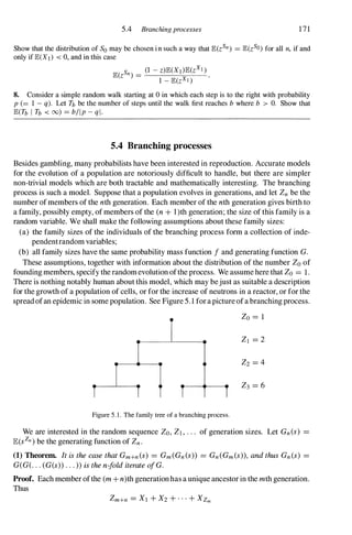
![172 5.4 Generatingfunctions and theirapplications
where Xi is the numberofmembers ofthe (m +n)th generation which stemfromthe i th mem
berofthemth generation. This is the sumofarandomnumber Zm ofvariables. These variables
are independent by assumption (a); furthermore, by assumption (b) they are identically dis
tributed with the same distribution as the number Zn of the nth-generation offspring of the
first individual in the process. Now use Theorem (5.1.25) to obtain Gm+n(s) = Gm(GXl (s»
where GXl (s) = Gn(s). Iterate this relation to obtain
and notice that Gl (s) is what we called G(s) . •
In principle, Theorem (1) tells us all about Zn and its distribution, but in practice Gn(s)
may be hard to evaluate. The moments of Zn, at least, may be routinely computed in terms
of the moments of a typical family size ZI . For example:
(2) Lemma. Let /L= lE(ZI) and a2 = var(ZI ). Then
{na2 if/L= 1,
lE(Zn) = /Ln, var(Zn) = a2(/Ln - 1)/Ln-l if/L=J. 1 .
/L- l
Proof. Differentiate Gn(s) = G(Gn-1 (s» once at s = 1 to obtain lE(Zn) = /LlE(Zn-l);by
iteration, lE(Zn) = /Ln. Differentiate twice to obtain
G�(l) = Gil(I)G�_1(1)2+G'(I)G�_1(1)
and use equation (5.1.19) to obtain the second result. •
(3) Example. Geometric branching. Suppose that each family size has the mass function
f(k) = qpk, for k � 0, where q = 1 - p. Then G(s) = q(1 - ps)- l , and each family size
is one member less than a geometric variable. We can show by induction that
{n - (n - l)s
n+ I - ns
Gn(s) = [ 1 1 ]
q pn _
qn _
ps(pn- _
qn-
)
pn+1 _
qn+l _
ps(pn _
qn)
'f 1
1 p = q = '2'
if p =J. q.
This result can be useful in providing inequalities for more general distributions. What can
we say about the behaviour of this process after many generations? In particular, does it
eventually become extinct, or, conversely, do all generations have non-zero size? For this
example, we can answer this question from a position of strength since we know Gn(s) in
closed form. In fact
n
if p = q,
n+l
q(pn_
qn)
pn+l _
qn+l if p =J. q.
Let n -+ 00 to obtain
{ I if p S q,
IP'(Zn = 0) -+ lP'(ultimate extinction) =
q/p if p > q.](https://image.slidesharecdn.com/grimmettstirzaker-probabilityandrandomprocessesthirded2001-220507085451-bb31ac14/85/Grimmett-Stirzaker-Probability-and-Random-Processes-Third-Ed-2001-pdf-183-320.jpg)
![5.4 Branching processes 173
We have used Lemma (1.3.5) here surreptitiously, since
(4) {ultimate extinction} = U{Zn = O}
n
and An = {Zn = O} satisfies An S; An+I' •
Wesawinthis example thatextinction occurs almost surely ifand only iff.J, = lEeZ1) = p/q
satisfies lE(ZI) ::s 1. This is a very natural condition; it seems reasonable that if lE(Zn) =
lEeZI)n ::s 1 then Zn = 0 sooner or later. Actually this result holds in general.
(5) Theorem. As n -+ 00, JP>(Zn = 0) -+ JP>(ultimate extinction) = 1'/, say, where 11 is the
smallest non-negative root oj the equation s = G(s). Also, 11 = 1 if f.J, < I, and 11 < 1
if f.J, > 1. IfjJ, = 1 then 11 = 1 so long as thejamily-size distribution has strictly positive
variance.
Prooft. Let 'f}n = IP'(Zn = 0). Then, by (1),
'f}n = Gn(O) = G(Gn-1(0» = G('f}n-t}.
In the light of the remarks about equation (4) we know that 'f}n t 'f},and the continuity of G
guarantees that 'f} = G('f}). We show next that if 1/1 is any non-negative root of the equation
s = G(s) then 'f} ::s 1/1. Note that Gis non-decreasing on [0, 1] and so
'f}I = G(O) ::s G(1/I) = 1/1.
Similarly
'f}2 = G('f}]) ::s G(1/I) = 1/1
and hence, by induction, 'f}n :'S 1/1 for all n, giving 'f} :'S 1/1. Thus 'f}is the smallest non-negative
root ofthe equation s = G(s).
To verify the second assertion ofthe theorem, we need the fact that Gis convex on [0, 1].
This holds because
So G is convex and non-decreasing on [0, 1] with G(l) = 1. We can verify that the two
curves y = G(s) and y = s generally have two intersections in [0, 1], and these occur at
s = 'f}and s = 1 . A glance at Figure 5.2 (and a more analytical verification) tells us that
these intersections are coincident if f.J, = G'(1) < 1. On the other hand, if f.J, > 1 then these
two intersections are not coincident. In the special case when f.J, = 1 we need to distinguish
between the non-random case in which 0'2 = 0, G(s) = s, and 'f} = 0, and the random case
in which 0'2 > 0, G(s) > s for O ::S s < 1, and 'f} = 1. •
tThis method of solution was first attempted by H. W. Watson in 1 873 in response to a challenge posed by
F. Galton in the April I edition of the Educational Times. For this reason, a branching process is sometimes
termed a 'Galton-Watson process'. The correct solution in modem format was supplied by J. F. Steffensen in
1930; I. J. Bienayme and J. B. S. Haldane had earlier realized what the extinction probability should be, but
failed to provide the required reasoning.](https://image.slidesharecdn.com/grimmettstirzaker-probabilityandrandomprocessesthirded2001-220507085451-bb31ac14/85/Grimmett-Stirzaker-Probability-and-Random-Processes-Third-Ed-2001-pdf-184-320.jpg)
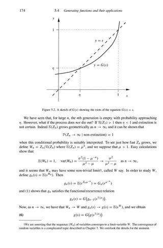
![5.5 Age-dependent branchingprocesses 175
by abandoning some ofour current notions ofmathematical rigour. This functional equation
can be established rigorously (see Example (7.8.5)) and has various uses. For example,
although we cannot solve it for g, we can reach such conclusions as 'if lE(Zf) < 00 then W
is continuous, apart from a point mass of size rJ at zero'.
We have made considerable progress with the theory of branching processes. They are
reasonably tractable because they satisfy the Markov condition (see Example (3.9.5)). Can
you formulate and prove this property?
Exercises for Section 5 .4
1. Let Zn be the size ofthe nthgenerationin an ordinary branchingprocess with Zo = 1, E(Z] ) = J-t,
and var(Z] ) > O. Show that E(ZnZm) = J-tn-mE(Z�) for m :s n. Hence find the correlation
coefficient p(Zm, Zn) in terms of J-t.
2. Consider a branching process with generation sizes Zn satisfying Zo = 1 and IP'(ZI = 0) = O.
Pick two individuals at random (with replacement) from the nth generation andlet L be the index of
the generation which contains their most recent common ancestor. Show that IP'(L = r) = E(Z;:-I) -
E(Z;�] ) for O :s r < n. What can be said if lP'(Z] = 0) > O?
3. Consider a branching process whose family sizes have the geometric mass function J(k) = qpk,
k :::: 0, where p + q = 1, and let Zn be the size of the nth generation. Let T = min{n : Zn = O} be
the extinction time, and suppose that Zo = 1. Find IP'(T = n). For what values of p is it the case that
E(T) < oo?
4. Let Zn be the size of the nth generation of a branching process, and assume Zo = 1. Find an
expression forthe generating function Gn of Zn, in the cases when Z] has generating function given
by:
(a) G(s) = l - a(l - s)f3, 0 < a, {3 < 1 .
(b) G(s) = J-I {P(f(s))}, where P is a probability generating function, and J is a suitable function
satisfying J(I) = 1.
(c) Supposeinthe latter case that J(x) = xm and pes) = sly - (y - l)s}-I where y > 1. Calculate
the answer explicitly.
5. Branching with immigration. Each generation ofabranching process (with a single progenitor)
is augmented by a random number of immigrants who are indistinguishable from the other members
ofthe popUlation. Suppose that the numbers of immigrants in different generations are independent
of each other and of the past history of the branching process, each such number having probability
generating function H (s). Show that the probability generating function Gn of the size of the nth
generation satisfies Gn+1 (s) = Gn (G(s»H(s), where G is the probability generating function of a
typical family of offspring.
6. Let Zn be the size of the nth generation in a branching process with E(sZJ ) = (2 - s)-]
and Zo = 1. Let Vr be the total number of generations of size r . Show that E(Vl) = in2, and
E(2V2 - V3) = in2 - Jon4.
5.5 Age-dependent branching processes
Here is a more general model forthe growth of a population. It incorporates the observation
thatgenerationsare not contemporaneousin mostpopUlations; in fact, individuals in the same
generation give birth to families at different times. To model this we attach another random
variable, called 'age', to each individual; we shall suppose that the collection of all ages is
a set of variables which are independent of each other and of all family sizes, and which](https://image.slidesharecdn.com/grimmettstirzaker-probabilityandrandomprocessesthirded2001-220507085451-bb31ac14/85/Grimmett-Stirzaker-Probability-and-Random-Processes-Third-Ed-2001-pdf-186-320.jpg)
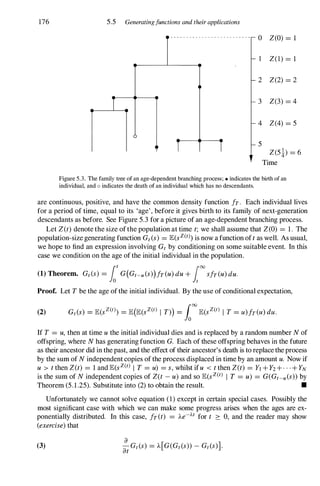
![180 5.6 Generatingfunctions and their applications
(b) (dominatedconvergence)if IXn (w)1 � Yew) for all n and w, and lElYI < 00, then
lE(Xn) -+ lE(X),
(c) (boundedconvergence, a special case of dominated convergence) if IXn(w)1 � cfor
some constant cand all n and w then lE(Xn) -+ lE(X).
Rathermore is true. Events having zero probability (that is, null events) make no contributions
to expectations, and may thereforebe ignored. Consequently, it suffices to assume abovethat
Xn (w) -+ X(w) for all w exceptpossibly on some null event, with a similar weakening
of the hypotheses of (a), (b), and (c). For example, the bounded convergence theorem is
normally stated as follows: if {Xn} is a sequence of random variables satisfying Xn -+ X
a.s. and IXn I � ca.s. for some constant c,then lE(Xn) -+ lE(X). The expression 'a.s.' is an
abbreviation for 'almost surely', and means 'except possibly on an event ofzero probability'.
Here is a useful consequence of monotone convergence. Let Zl , Z2, . . . be non-negative
random variables with finite expectations, and let X = L�l Zi. We have by monotone
convergence applied to the partial sums ofthe Zi that
00
(13) lE(X) = LlE(Zi),
i=1
whether ornotthe summation is finite.
One further property of expectation is called Fatou's lemma: if {Xn} is a sequence of
random variables such that Xn 2: Y a.s. for all nand some Y with lElYI < 00, then
(14) lE(lim inf Xn) � lim inf lE(Xn).
n---+oo n---+oo
This inequality is often applied in practice with Y = o.
(15) Lebesgue-Stieltjes integral. Let X have distribution function F. The function F gives
rise to a probability measure J-LF on the Borel sets of JR as follows:
(a) define J-LF ( a,bl) = F(b)-F(a),
(b) asin the discussion after (4.1.5), the domain ofJ-LF can be extended to include the Borel
a-field $ , being the smallest a-field containing all half-open intervals (a,b].
So (JR, $ , J-LF) is a probability space; its completion (see Section 1.6) is denoted by the
triple (JR, £F , J-LF), where £F is the smallest a-field containing $ and all subsets of J-LF
null sets. If g : JR -+ JR (is £F-measurable) then the abstract integral J gdJ-LF is called the
Lebesgue-Stieltjesintegralof gwith respect to J-LF, and we normally denote it by J g(x)dF
or J g(x)dF(x). Think of it as a special case of the abstract integral (1 1). The purpose of
this discussion is the assertion that if g : JR -+ JR (and gis suitably measurable) then g(X) is
random variable and
lE(g(X» = !g(x)dF,
and we adopt this forthwith as the official notation for expectation. Here is a final word of
caution. If g(x) = IB(X)h(x)where IBis the indicator function of some B S; JR then
!g(x)dF= Ish(x)dF.
Wedonotingeneral obtain the sameresult when we integrate over Bl = [a,b]and B2 = (a,b)
unless Fis continuous at aand b,and so we do not use the notation J: h(x)dFunless there
is no danger of ambiguity.](https://image.slidesharecdn.com/grimmettstirzaker-probabilityandrandomprocessesthirded2001-220507085451-bb31ac14/85/Grimmett-Stirzaker-Probability-and-Random-Processes-Third-Ed-2001-pdf-191-320.jpg)
![182 5.7 Generatingfunctions and their applications
(c) if X and Y are independent thent Mx+Y(t) = Mx(t)My(t).
Moment generating functions provide a very useful technique but suffer the disadvantage
that the integrals which define them may not always be finite. Rather than explore their
properties in detail we move on immediately to another class of functions that are equally
useful and whose finiteness is guaranteed.
(2) Definition. The characteristic function of X is the function rP : III -+ C defined by
rP(t) = E(eitx) where i = P.
We often write ¢x forthe characteristic function ofthe random variable X. Characteristic
functions are related to Fourier transforms, since ¢(t) = J eitxdF(x). In the notation of
Section 5.6, ¢is the abstractintegral of a complex-valued random variable. It is well defined
in the terms of Section 5.6 by ¢(t) = lE(cos tX) + ilE(sin tX). Furthermore, ¢ is better
behaved than the moment generating function M.
(3) Theorem. Thecharacteristicfunction¢satisfies:
(a) ¢(O) = 1, 1¢(t)1 .s 1 forallt,
(b) ¢isuniformlycontinuousonlR,
(c) ¢ is non-negativedefinite, which is tosay that Lj,k¢(tj - tk)Z/Zk 2: 0 forallreal
tl,t2,... ,tnandcomplexZI,Z2,... ,Zn·
Proof. (a) Clearly ¢(O) = lE(l) = 1. Furthermore
1¢(t)1 .s f leitxl dF = fdF = 1.
(b) We have that
where Y(h) = leihX -l l. However, IY(h)l .s 2 and Y(h) -+ O as h -+ O, and solE(Y(h» -+ 0
by bounded convergence (5.6.12).
(c) We have that
L¢(tj -tk)Z/Zk = Lf[Zjexp(itjx)][Zkexp(-itkX)]dF
hk hk
= lE(I�>jexp(itjX) 12) 2: O.
]
•
Theorem (3) characterizes characteristic functions in the sense that ¢ is a characteristic
function ifand only ifit satisfies (3a), (3b), and (3c). This result is called Bochner's theorem,
for which we offer no proof. Many of the properties ofcharacteristic functions rely fortheir
proofs pn a knowledge ofcomplex analysis. This is a textbook on probability theory, and will
tThis is essentially the assertion that the Laplace transfonn of a convolution (see equation (4.8.2» is the
product of the Laplace transfonns.](https://image.slidesharecdn.com/grimmettstirzaker-probabilityandrandomprocessesthirded2001-220507085451-bb31ac14/85/Grimmett-Stirzaker-Probability-and-Random-Processes-Third-Ed-2001-pdf-193-320.jpg)
![5.7 Characteristicfunctions 183
not include such proofs unless they indicate some essential technique. We have asserted that
the method of characteristic functions is very useful; however, we warn the reader that we
shall not make use of them until Section 5.10. In the meantime we shall establish some of
their properties.
First and foremost, from a knowledge of ¢x we can recapture the distribution of X. The
full power of this statement is deferred until the next section; here we concern ourselves only
with the moments of X. Several ofthe interesting characteristic functions are not very well
behaved, and we must move carefully.
(4) Theorem.
{ lElXkl < 00
(a) Ij¢(k)(O) exists then k 1
lElX - 1 < 00
(b) IjlElXkl < 00 thent
ifk is even,
ifk is odd.
Proof. This is essentially Taylor's theorem for a function of a complex variable. For the
proof, see Moran (1968) or Kingman and Taylor (1966). •
One ofthe useful properties ofcharacteristic functions is thatthey enable us to handle sums
ofindependent variables with the minimum of fuss.
(5) Theorem. IfX and Y are independent then ¢x+y(t) = tPx(t)t/>y(t).
Proof. We have that
¢X+Y(t) = lE(eit(x+y» = lE(eitXeitY).
Expand each exponential term into cosines and sines, multiply out, use independence, and put
back together to obtain the result. •
(6) Theorem. Ifa, b E IR and Y = aX + b then ¢y(t) = eitb¢x(at).
Proof. We have that
¢y(t) = lE(eit(aX+b» = lE(eitbei(at)X)
= eitblE(ei(at)X) = eitb¢x(at). •
We shall make repeated use of these last two theorems. We sometimes need to study
collections ofvariables which may be dependent.
(7) Definition. Thejointcharacteristicfunction ofX and Y is the function ¢X,Y : ]R2 � ]R
given by ¢X,y(s, t) = lE(eisXeitY).
Notice that¢x,Y(s, t) = ¢sx+ty(1). As usual we shallbeinterested mostly in independent
variables.
tSee Subsection (10) of Appendix I for a reminder about Landau's % notation.](https://image.slidesharecdn.com/grimmettstirzaker-probabilityandrandomprocessesthirded2001-220507085451-bb31ac14/85/Grimmett-Stirzaker-Probability-and-Random-Processes-Third-Ed-2001-pdf-194-320.jpg)
![184 5.7 Generatingfunctions and their applications
(8) Theorem. RandomvariablesX andYareindependentifandonlyif
¢X,y(s,t) = ¢x(s)¢y(t) forallsandt.
Proof. If X and Yare independent then the conclusion follows by the argument of (5). The
converse is proved by extending the inversion theorem of the next section to deal with joint
distributions and showing that thejoint distribution function factorizes. •
Note particularly that for X and Yto be independent it is not sufficient that
(9) ¢X,y(t,t) = ¢x(t)¢y(t) for all t.
Exercise. Can you find an example of dependent variables which satisfy (9)?
We have seen in Theorem (4)that it is an easy calculation to find the moments of X by
differentiating its characteristic function ¢x(t)at t = O. A similar calculation gives the 'joint
moments' JE(xj yk) of two variables from a knowledge of their joint characteristic function
¢X,y(s,t) (see Problem (5.12.30)for details).
The properties ofmomentgeneratingfunctions are closely relatedtothose ofcharacteristic
functions. In the rest of the text we shall use the latter whenever possible, but it will be
appropriate to use the former for any topic whose analysis employs Laplace transforms; for
example, this is the case for the queueing theory of Chapter 11.
(10) Remark. Moment problem. If! am given a distribution function F,then I can calculate
the corresponding moments mk(F) = f�
oo xkdF(x),k= 1,2,. . . , whenever these integrals
exist. Is the converse true: does the collection of moments (mk(F) :k= 1,2,. .. ) specify F
uniquely? The answer is no: there existdistribution functions Fand G, all ofwhose moments
exist, such that F =1=G but mk(F) = mk(G) forall k. The usual example is obtained by using
the log-normal distribution (see Problem (5.12.43».
Under what conditions on F is it the case thatno such G exists? Various sets ofconditions
are known which guaranteethat Fis specified by its moments, butno necessary and sufficient
condition is known which is easy to apply to a general distribution. Perhaps the simplest
sufficient condition is that the moment generating function of F, M(t) = f�
oo etx dF(x),be
finite in some neighbourhood of the point t = O. Those familiar with the theory of Laplace
transforms will understand why this is sufficient.
(11) Remark. Moment generating function. The characteristic function ofa distribution is
closely related to its momentgenerating function, in amannermaderigorous in the following
theorem, the proof of which is omitted. [See Lukacs 1970,pp. 197-198.]
(12) Theorem. LetM(t) = JE(etx), t E JR, and¢(t) = JE(eitX), t E C, be themoment
generatingfunctionandcharacteristicfunction, respectively, ofarandomvariableX. For
anya > 0, thefollowingthreestatementsareequivalent:
(a) IM(t)1 < ooforItI < a,
(b) ¢isanalyticonthestrip Ilm(z)1 < a,
(c) themomentsmk = JE(Xk) existfork= 1,2,. . . andsatisfYlim suPk--->OO {lmkl/k!}
Ilk :s
a-I.
If any of these conditions hold for a > 0, the power series expansion for M(t) may be
extended analytically to the strip Ilm(t)I < a,resulting in a function Mwith the propertythat
¢(t) = M(it). [See Moran 1968,p. 260.]](https://image.slidesharecdn.com/grimmettstirzaker-probabilityandrandomprocessesthirded2001-220507085451-bb31ac14/85/Grimmett-Stirzaker-Probability-and-Random-Processes-Third-Ed-2001-pdf-195-320.jpg)
![186 5.8 Generatingjunctions and their applications
10. If X and Y are continuous random variables, show that
L:¢x (y) !y (y)e-ity dy = L:¢y (x - t)!x (x) dx.
11. Tilted distributions. (a) Let X have distribution function F and let r be such that M(r) =
JE.(e'x) < 00. Show that F. (x) = M(r)-l J�oo e'Y dF(y) is a distribution function, called a 'tilted
distribution' of X, and find its moment generating function.
(b) Suppose X and YareindependentandJE.(e'x ), JE.(e' Y) < 00. Findthemomentgeneratingfunction
of the tilted distribution of X + Y in terms of those of X and Y.
5.S Examples of characteristic functions
Those who feel daunted by i = R should find it a useful exercise to work through this
section using M(t) = JE(etx) in place of ¢(t) = JE(eitX). Many calculations here are left as
exercises.
(1) Example. Bernoulli distribution. If X is Bernoulli with parameter p then
•
(2) Example. Binomial distribution. If X is bin(n, p) then X has the same distribution as
the sum ofn independent Bernoulli variables Yl , Y2, . . . , Yn. Thus
(3) Example. Exponential distribution. If f(x) = Ae-Ax for x 2: 0 then
•
This is a complex integral and its solution relies on a knowledge of how to integrate around
contoursin]R2 (the appropriate contourisa sector). Alternatively, the integral maybeevaluated
by writing eitx = cos(tx) + i sin(tx), and integrating the real and imaginary part separately.
Do not fall into the trap oftreating i as ifits were a real number, even though this malpractice
yields the correct answer in this case:
A
¢(t) = --
. .
A - I t
(4) Example. Cauchy distribution. If f(x) = 1/{JT(1 + x2)} then
1 100 eitx
¢(t) = - --
2 dx.
JT -00 1 + x
•](https://image.slidesharecdn.com/grimmettstirzaker-probabilityandrandomprocessesthirded2001-220507085451-bb31ac14/85/Grimmett-Stirzaker-Probability-and-Random-Processes-Third-Ed-2001-pdf-197-320.jpg)
![5.8 Examples ofcharacteristicjunctions 187
Treating i as a real number will not help you to avoid the contour integral this time. Those
who are interested should try integrating around a semicircle with diameter [- R, R] on the
real axis, thereby obtaining the required characteristic function ¢(t) = e-1tl• Alternatively,
you might work backwards from the answer thus: you can calculate the Fourier transform of
the function e-1tl,and then use the Fourier inversion theorem. •
(5) Example. Normal distribution. If Xis N(O, 1) then
. 100 1
¢(t) = JE(e1tX) = J;L exp(itx- !x2)dx.
-00 v2n
Again, do not treat ias areal number. Consider instead the momentgenerating function of X
100 1
M(s) = JE(eSx) = J;L exp(sx- !x2)dx.
-00 v2n
Complete the square in the integrand and use the hint at the end ofExample (4.5.9) to obtain
M(s) = e�s2. We may not substitute s = itwithoutjustification. In this particular instance
thetheory ofanalytic continuationoffunctions ofacomplex variableprovidesthisjustification,
see Remark (5.7.1 1), and we deduce that
By Theorem (5.7.6), the characteristic function ofthe N(J-L,a2)variable Y = aX+ J-Lis
¢y(t) = eitfL¢x(at) = exp(iJ-Lt- !a2t2). •
(6) Example. Multivariate normal distribution. If Xl,X2,... ,Xn has the multivariate
normal distribution N(0, V) then its joint density function is
The joint characteristic function of XI,X2,... ,Xn is the function ¢(t) = JE(eitX') where
t = (tl,t2,... ,tn) and X = (XI , X2,... ,Xn). One way to proceed is to use the fact that
tX' is univariate normal. Alternatively,
(7)
As in the discussion of Section 4.9, there is a linear transformation y = xB such that
V-I , ,"" 2
X X = �AjYj
j
just as in equation (4.9.3). Make this transformation in (7) to see that the integrand factorizes
into the product of functions ofthe single variables Yl,Y2,... ,Yn. Then use (5) to obtain
¢(t) = exp(-!tVt').](https://image.slidesharecdn.com/grimmettstirzaker-probabilityandrandomprocessesthirded2001-220507085451-bb31ac14/85/Grimmett-Stirzaker-Probability-and-Random-Processes-Third-Ed-2001-pdf-198-320.jpg)
![5.9 Inversion and continuity theorems 189
10. Is it possible for X, Y, and Z to have the same distribution and satisfy X = U(Y + Z), where
U is uniform on [0, 1 ], and Y, Z are independent of U and of one another? (This question arises in
modelling energy redistribution among physical particles.)
11. Findthejointcharacteristicfunctionoftworandomvariables having abivariatenormaldistribution
with zero means. (No integration is needed.)
5.9 Inversion and continuity theorems
This section contains accounts oftwo major ways in which characteristic functions are useful.
The firstofthese states thatthe distribution ofarandomvariableis specified by its characteristic
function. That is to say, if X and Y have the same characteristic function then they have
the same distribution. Furthermore, there is a formula which tells us how to recapture the
distribution function F corresponding to the characteristic function ¢. Here is a special case
first.
(1) Theorem. IfX is continuous with densityfunction fand characteristicfunction ¢ then
f(x) = - e-ztx¢(t) dt
1 100 .
2rc -00
at every pointxat which fis differentiable.
Proof. This is the Fourier inversion theorem and can be found in any introduction to Fourier
transforms. Ifthe integral fails to converge absolutely then we interpretit as its principal value
(see Apostol 1974, p. 277). •
A sufficient, butnot necessary conditionthatacharacteristic function¢ be the characteristic
function of a continuous variable is that
i: 1¢(t)1 dt < 00.
The general case is more complicated, and is contained in the next theorem.
(2) Inversion theorem. Let X have distributionfunction F and characteristicfunction ¢.
Define F : lR -? [0, 1] by
Then
F(x) = � {F(X) + lim F(Y) }.
2 ytx
F(b) - F(a) = lim
e -
.
e
¢(t) dt.
I
N -iat -ibt
N-+oo -N 2rclt
Proof. See Kingman and Taylor (1966). •
(3) Corollary. Random variables X and Y have the same characteristicfunction ifandonly
ifthey have the same dtstrlbutionfunction.
Proof. If ¢x = ¢y then, by (2),
Fx(b) - Fx(a) = Fy(b) - FrCa).](https://image.slidesharecdn.com/grimmettstirzaker-probabilityandrandomprocessesthirded2001-220507085451-bb31ac14/85/Grimmett-Stirzaker-Probability-and-Random-Processes-Third-Ed-2001-pdf-200-320.jpg)
![5.9 Inversion and continuity theorems
A more general form of this relation states that
(7)
ret)
----== -+ 1 as t-+ 00
tt-Ie-t,.j2rct
191
where ris the gamma function, ret) = 1000 xt-1e-X dx. Remember that ret) = (t- I ) ! if t
is a positive integer; see Example (4.4.6) and Exercise (4.4.1). To prove (7) is an 'elementary'
exercise in analysis, (see Exercise (5.9.6» , but it is perhaps amusing to see how simply (7)
follows from the Fourier inversion theorem (1).
Let Y bearandomvariable with the r(l,t)distribution. Then X = (Y -t)/,Jthas density
function
(8) ft(x) = _1-../t(x../t+t)t-l exp[-(x../t+t)], -../tS x < 00,
ret)
and characteristic function
Now ft(X)is differentiable with respect to x on (-,Jt,00). We apply Theorem (1) at x = 0
to obtain
(9)
1
100
ft(O) = - ¢t(u)du.
2rc -00
However, fl(O) = tt-�e-f/ret)from (8); also
¢t(u) = exp [-iu../t-tlog (1 - �)]
= exp [-iU../t-t(-�+ ;;+O(U3t-� »)]
= exp[- !u2 +O(u3t-�)] -+ e-�u
2
as t -+ 00.
Taking the limit in (9) as t -+ 00, we find that
lim __ tt-"2e-t = lim - ¢t(u)du
( 1 1
) 1
100
t---+oo ret) t---+oo 2rc -00
= _
1
100 (lim ¢t(U»)du
2rc -00
t---+oo
as required for (7). A spot of rigour is needed to justify the interchange of the limit and the
integral sign above, and this may be provided by the dominated convergence theorem. •](https://image.slidesharecdn.com/grimmettstirzaker-probabilityandrandomprocessesthirded2001-220507085451-bb31ac14/85/Grimmett-Stirzaker-Probability-and-Random-Processes-Third-Ed-2001-pdf-202-320.jpg)
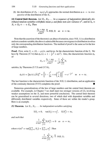
![5.10 Two limit theorems 195
Proof. See Loeve (1977,p. 287),and also Problem (5.12.40). •
The roots of central limit theory are at least 250years old. The first proofof (4)was found
by de Moivre around 1733for the special case of Bernoulli variables with p = �. General
values of p were treated later by Laplace. Their methods involved the direct estimation of
sums ofthe form
L
k:
k�np+xy'njiii
where p + q = 1.
The first rigorous proofof (4)was discovered by Lyapunov around 1901,thereby confirming
a less rigorous proof of Laplace. A glance at these old proofs confirms that the method of
characteristic functions is outstanding in its elegance and brevity.
Thecentral limittheorem (4)asserts thatthedistributionfunctionofSn, suitably normalized
to have mean 0and variance 1,converges to the distribution function ofthe N(O, 1)distribu
tion. Is the corresponding result valid at the level of density functions and mass functions?
Broadly speaking the answer is yes, but some condition of smoothness is necessary; after all,
if Fn(x) -+ F(x) as n-+ 00 forall x, it is not necessarily the case that the derivatives satisfy
F�(x) -+ F'(X). [See Exercise (5.9.2).] The result which follows is called a 'local central
limit theorem' since it deals in the local rather than in the cumulative behaviour ofthe random
variables in question. In order to simplify the statement ofthe theorem, we shall assume that
the Xi have zero mean and unit variance.
(6) Local central limit theorem. LetXI , X2, ... beindependentidenticallydistributedran
dom variables with zero meanandunitvariance, andsupposefurtherthat theircommon
characteristicfunction¢satisfies
(7) i:1¢(tWdt < 00
forsomeintegerr :::: 1. ThedensityfunctiongnofUn = (XI + X2 + . . . + Xn)/Inexists
forn ::::r,andfurthermore
1 1 2
(8) gn(x) -+ �e-"2x asn -+ 00, uniformlyinx E K
v2n
A similar result is valid for sums of lattice-valued random variables, suitably adjusted to
have zero mean and unit variance. We state this here, leaving its proof as an exercise. In place
of (7)we assume that the Xi are restricted to take the values a,a ± h,a ± 2h, . . . , where
his the largest positive number for which such a restriction holds. Then Un is restricted to
values of the form x = (na + kh)/Infor k = 0,±1, . . . . For such a number x, we write
gn(x) = JP>(Un = x) and leave gn(Y)undefined for other values of y. It is the case that
(9)
In 1 l X2
-gn(x) -+ --e-"2 as n -+ 00, uniformly in appropriate x.
h .[iii
Proofof (6). A certain amount of analysis is inevitable here. First, the assumption that 1¢lr
is integrable for some r :::: 1implies that I¢Inis integrable for n ::::r,since I¢(t)l S I ; hence
gn exists and is given by the Fourier inversion formula
(10) gn(x) = - e-ztx1/In(t)dt,
1 100
.
2n -00](https://image.slidesharecdn.com/grimmettstirzaker-probabilityandrandomprocessesthirded2001-220507085451-bb31ac14/85/Grimmett-Stirzaker-Probability-and-Random-Processes-Third-Ed-2001-pdf-206-320.jpg)
![196 S.10 Generatingfunctions and their applications
where 1/In(t) = ¢(t/,/nf is the characteristic function of Un. The Fourierinversion theorem
is valid for the normal distribution, and therefore
(11)
where
In = _
1
/00I¢(t,/fi)n _e-!t21dt.
2n -00
It suffices to show that In � 0 as n � 00. We have from Theorem (S.7.4) that ¢(t) =
1 - it2+0(t2)as t � 0, and therefore there exists 8 (> 0) such that
(12)
Now, for any a > O,¢(t/...(ii)n � e-!t2 as n � oo uniformly in t E [-a, a] (to see this,
investigate the proofof (4) slightly more carefully), so that
(13)
for any a. Also, by (12),
(14)
which tends to zero as a � 00.
It remains to deal with the contribution to In arising from ItI > 8...(ii. From the fact that
gn exists for n � r , we have from Exercises (S.7.S) and (S.7.6) that 1¢(tYI < 1 for t =f:. 0,
and 1¢(tYI � 0 as t � ±oo. Hence 1¢(t)1 < 1 for t =f:. 0, and 1¢(t)1 � 0 as t� ±oo, and
therefore 1/ = sup{l¢(t) I : ItI � 8} satisfies 1/ < 1 . Now, for n � r ,
(15) [ 1¢(t/...(ii)n _e-!t2Idt S 1/n-r/00 1¢(t/...(iiWdt+2 [00 e-!t2dt
J1tl>8.jTi -00 J8.jTi
Combining (13)-(1S), we deduce that
so that In � 0 as n � 00 as required.
= 1/n-r...(ii/oo
1¢(uWdu+2 [00 e-!t2dt
-00 J8.jTi
� 0 as n � 00.
as a � 00,
•
(16) Example. Random walks. Here is an application of the law of large numbers to the
persistence of random walks. A simple random walk performs steps of size 1, to the right
or left with probability p and 1 - p. We saw in Section S.3 that a simple random walk is
persistent (that is, returns to its starting point with probability 1) ifand only ifit is symmetric](https://image.slidesharecdn.com/grimmettstirzaker-probabilityandrandomprocessesthirded2001-220507085451-bb31ac14/85/Grimmett-Stirzaker-Probability-and-Random-Processes-Third-Ed-2001-pdf-207-320.jpg)
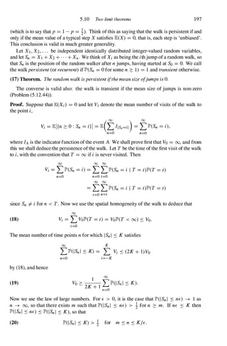
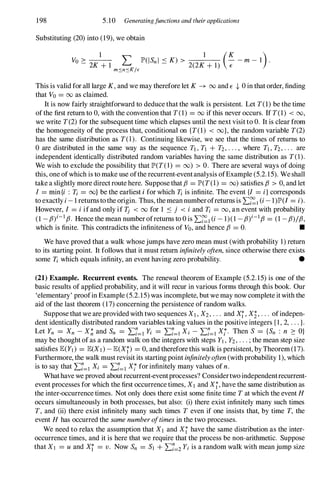
![5.1 1 Large deviations 201
[Hint: Use the result of Problem (5. 12. 1 8).]
8. Let {Xr : r 2: I } be independent with the distribution of the preceding Exercise (7). Let
Un = n-I L:�=I Xr, and Tn = n-1Un. Show that:
(a) JP'(Un < c) -7 0 for any c < 00,
(b) Tn has the same distribution as XI .
9. A sequence of biased coins is flipped; the chance that the rth coin shows a head is 8r, where 8r
is a random variable taking values in (0, 1). Let Xn be the number of heads after n flips. Does Xn
obey the central limit theorem when:
(a) the 8r are independent and identically distributed?
(b) 8r = 8 for all r, where 8 is a random variable taking values in (0, I)?
5.11 Large deviations
Thelaw oflargenumbersassertsthat,in acertain sense, the sum Sn ofnindependentidentically
distributedvariables is approximately nf-t, where f-t is atypicalmean. Thecentral limittheorem
implies thatthe deviations ofSn fromnf-t are typically ofthe order In, that is, small compared
with the mean. Now, Sn may deviate from nf-t by quantities of greater order than In, say nCi
where CL > 1, but such 'large deviations' have probabilities which tend to zero as n � 00.
Itis often necessary in practice to estimate such probabilities. The theory oflarge deviations
studies the asymptotic behaviour ofIP'(ISn -nf-t I > nCi)as n � 00, for values ofCL satisfying
CL > 1; of particular interest is the case when CL = 1, corresponding to deviations of Sn from
its mean nf-t having the same order as the mean. The behaviourofsuch quantities is somewhat
delicate, depending on rathermore than the mean and variance of a typical summand.
LetXl, X2, . . . be a sequence ofindependentidentically distributedrandomvariables with
mean f-t and partial sums Sn = Xl + X2 + . . . + Xn. It is our target to estimate IP'(Sn > na)
where a > f-t. The quantity central to the required estimate is the moment generating function
M(t) = JE(etx) of a typical Xi, or more exactly its logarithm A(t) = log M(t). The function
A is also known as the cumulantgeneratingfunctionof the Xi (recall Exercise (5.7.3» .
(1)
Before proceeding, we note some properties of A. First,
A(O) = log M(O) = 0,
M'(O)
A'(0) = -- = if M'(0) exists.
M(O)
f-t
Secondly, A(t)is convex wherever it is finite, since
(2) A"(t) =
M(t)M"(t)-M'(t)2
M(t)2
JE(etX)JE(X2etX) _ JE(XetX)2
M(t)2
which is non-negative, by the Cauchy-Schwarz inequality (4.5.12) applied to the random
variables Xe!tX and e!tx. We define the Fenchel-Legendretransform of A(t) to be the
function A*(a)given by
(3) A*(a)= sup{at -A(t)},
tEIR
a E K
The relationship between A and A* is illustrated in Figure 5.4.](https://image.slidesharecdn.com/grimmettstirzaker-probabilityandrandomprocessesthirded2001-220507085451-bb31ac14/85/Grimmett-Stirzaker-Probability-and-Random-Processes-Third-Ed-2001-pdf-212-320.jpg)
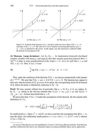
![206 5.12 Generatingfunctions and their applications
Exercises for Section 5 . 1 1
1. A fair coin is tossed n times, showing heads Hn times and tails Tn times. Let Sn = Hn - Tn.
Show that
IP'(Sn > an) l/n ---+ if 0 < a < 1.
J(1 + a) 1+a( 1 - a) l-a
What happens if a 2: I ?
2. Show that
r,l/n 4
n ---+ -----r===.=:;====;==
)(1 + a) 1+a( 1 - a) l-a
as n ---+ 00, where 0 < a < 1 and
Tn = � (�).
Ik-inl>�an
Find the asymptotic behaviour of Tnl/n where
Tn = L
k:
k>n(l+a)
where a > O.
3. Show that the moment generating function of X is finite in a neighbourhood of the origin if and
only if X has exponentially decaying tails, in the sense that there exist positive constants A and /-L such
that 1P'(I X I 2: a) ::s /-Le-J...a for a > O. [Seen in the light of this observation, the condition of the large
deviation theorem (5.11.4) is very natural].
4. Let Xl , X2 , ' " be independent random variables having the Cauchy distribution, and let Sn =
Xl + X2 + . . . + Xn. Find lP'(Sn > an).
5.12 Problems
1. A die is thrown ten times. What is the probability that the sum of the scores is 27?
2. A coin is tossed repeatedly, heads appearing with probability p on each toss.
(a) Let X be the number of tosses until the first occasion by which three heads have appeared
successively. Write down a difference equation for f(k) = IP'(X = k) and solve it. Now write
down an equation for IE(X) using conditional expectation. (Try the same thing for the first
occurrence of HTH).
(b) Let N be the number of heads in n tosses of the coin. Write down GN(S). Hence find the
probability that: (i) N is divisible by 2, (ii) N is divisible by 3.
3. A coin is tossed repeatedly, heads occurring on each toss with probability p. Find the probability
generating function of the number T of tosses before a run of n heads has appeared for the first time.
4. Find the generating function of the negative binomial mass function
f(k) = (k - 1)pr(1 _
p)k-r,
r - 1
k = r, r + 1, . . . ,](https://image.slidesharecdn.com/grimmettstirzaker-probabilityandrandomprocessesthirded2001-220507085451-bb31ac14/85/Grimmett-Stirzaker-Probability-and-Random-Processes-Third-Ed-2001-pdf-217-320.jpg)
![208 5.12 Generatingfunctions and their applications
14. The distribution of a random variable X is called infinitely divisible if, for all positive integers n,
there exists a sequence Y?), yin), . . . , y�n) of independent identically distributed random variables
such that X and yl(n) + yt) + . . . + y�n) have the same distribution.
(a) Show that the normal, Poisson, and gamma distributions are infinitely divisible.
(b) Show that the characteristic function </> of an infinitely divisible distribution has no real zeros, in
that </> (t) I=- 0 for all real t.
15. Let XI, X2, . .. be independent variables each taking the values 0or 1 with probabilities 1 -p and
p, where 0 < p < 1. Let N be a random variable taking values in the positive integers, independent
of the Xi, and write S = XI + X2 + . . . + XN . Write down the conditional generating function of N
given that S = N, in terms of the probability generating function G of N. Show that N has a Poisson
distribution if and only if IE(xN)P = IE(xN I S = N) for all p and x.
16. If X and Y have joint probability generating function
where PI + P2 ::::: 1,
find the marginal mass functions of X and Y, and the mass function of X+ Y. Find also the conditional
probability generating function GXIY(s I y) = IE(sX I Y = y) of X given that Y = y. The pair X, Y
is said to have the bivariate negative binomial distribution.
17. If X and Y have joint probability generating function
GX,Y(s, t) = exp{ex(s - 1) + {J(t - 1) + y(st - I)}
find the marginal distributions of X, Y, and the distribution of X + Y, showing that X and Y have the
Poisson distribution, but that X + Y does not unless y = O.
18. Define
for a, b > O. Show that
(a) I(a, b) = a-I1(1, ab), (b) al /ab = -2/(1, ab),
(c) I(a, b) = .fife-2ab/(2a).
(d) If X has density function (d/'/x)e-c/x-gx for x > 0, then
IE(e-tX) = dV 71: exp (-2vc(g + t)) , t > -g.
g + t
1
(e) If X has density function (271:x3)- 2: e-I/(2x) for x > 0, then X has moment generating function
given by IE(e-tX) = exp{-J2t}, t 2: O. [Note that IE(Xn) = 00 for n 2: 1.]
19. Let X, Y, Z be independent N(O, 1) variables. Use characteristic functions and moment gener
ating functions (Laplace transforms) to find the distributions of
(a) U = X/Y,
(b) V = X-2,
(c) W = XYZ/VX2y2 + Y2Z2 + Z2X2.
20. Let Xhave density function f and characteristic function </>, and suppose that J::'ooI</>(t)I dt < 00.
Deduce that
f(x) = - e-ztx</> (t) dt.
1 100 .
271: -00
21. Conditioned branching process. Consider a branching process whose family sizes have the
geometric mass function f(k) = qpk, k 2: 0, where /l, = p/q > 1. Let Zn be the size of the nth](https://image.slidesharecdn.com/grimmettstirzaker-probabilityandrandomprocessesthirded2001-220507085451-bb31ac14/85/Grimmett-Stirzaker-Probability-and-Random-Processes-Third-Ed-2001-pdf-219-320.jpg)
![210 5.12 Generatingfunctions and their applications
32. Let XI , X2, . . . be independent variables which are uniformly distributed on [0, 1 ]. Let Mn =
max{XI , X2, . . . , Xn} and show that n(1 - Mn) � X where X is exponentially distributed with
parameter 1 . You need not use characteristic functions.
33. If X is either (a) Poisson with parameter A, or (b) 1'( 1 , A), show that the distribution of fA =
(X - EX)/"jvar X approaches the N(0, 1 ) distribution as A ---+00.
(c) Show that
e-n 1 + n + - + . . . + - ---+ -
( n2 nn ) 1
2! n! 2
as n ---+00.
34. Coupon collecting. Recall that you regularly buy quantities of some ineffably dull commodity.
To attract your attention, the manufacturers add to each packet a small object which is also dull, and in
addition useless, but there are n different types. Assume that each packet is equally likely to contain
any one of the different types, as usual. Let Tn be the number of packets bought before you acquire
a complete set of n objects. Show that n-I(Tn - n log n) � T, where T is a random variable with
distribution function IP'(T .:'0 x) = exp(-e-X), -00 < x < 00.
35. Find a sequence (¢n) ofcharacteristic functions with the property that the limit given by ¢(t) =
limn---+00 ¢n (t) exists for all t, but such that ¢ is not itself a characteristic function.
36. Use generating functions to show that it is not possible to load two dice in such a way that the
sum of the values which they show is equally likely to take any value between 2 and 1 2. Compare
with your method for Problem (2.7. 1 2).
37. A biased coin is tossed N times, where N is a random variable which is Poisson distributed
with parameter A. Prove that the total number of heads shown is independent of the total number of
tails. Show conversely that ifthe numbers of heads and tails are independent, then N has the Poisson
distribution.
38. A binary tree is a tree (as in the section on branching processes) in which each node has exactly
two descendants. Suppose that each node of the tree is coloured black with probability p, and white
otherwise, independently of all other nodes. For any path n containing n nodes beginning at the root
of the tree, let B(n) be the number ofblack nodes in n , and let Xn(k) be the number of such paths n
for which B(n) � k. Show that there exists f3e such that
E{Xn(f3n)} ---+ { O �f f3 > f3e,
00 If f3 < f3e,
and show how to determine the value f3e.
Prove that
(
) { 0 if f3 > f3e,
II" Xn(f3n) � 1 ---+ 1 if f3 < f3e.
39. Use the continuity theorem (5.9.5) to show that, as n ---+00,
(a) if Xn is bin(n, A/n) then the distribution of Xn converges to a Poisson distribution,
(b) if Yn is geometric with parameter p = A/n then the distribution of Yn/n converges to an expo
nential distribution.
40. Let XI , X2, . . . be independent random variables with zero means and such that EIXJI < 00 for
all j. Show that Sn = XI + X2 + . . . + Xn satisfies Sn/"jvar(Sn) � N(O, 1 ) as n ---+00 if
The following steps may be useful. Let u/ = var(Xj), u(n)2 = var(Sn), Pj = ElxJI, and ¢j
and 1/In be the characteristic functions of Xj and Sn/u(n) respectively.](https://image.slidesharecdn.com/grimmettstirzaker-probabilityandrandomprocessesthirded2001-220507085451-bb31ac14/85/Grimmett-Stirzaker-Probability-and-Random-Processes-Third-Ed-2001-pdf-221-320.jpg)
![216 6.1 Markov chains
Proof. We have that
I-Lt+n) = IP'(Xm+n = j) = LIP'(Xm+n = j I Xm = i)lP'(Xm = i)
i
and the result follows from Theorem (7). •
Thus we reach the importantconclusionthatthe random evolutionofthe chain is determined
by the transition matrix P and the initial mass function JL(0). Many questions about the chain
can be expressedin terms ofthese quantities, and the study ofthe chain is thuslargelyreducible
to the study of algebraic properties of matrices.
(9) Example. Simple random walk. The simple random walk on the integershas state space
S= {a, ±1, ±2, ...}and transition probabilities
if j = i + l,
if j = i - I,
otherwise.
The argument leading to equation (3.10.2) shows that
{ (1
n
. . )p�(n+j-i)q�(n-j+i)
Pij(n) = z(n + ] -z )
°
if n + j - i is even,
otherwise.
•
(10) Example. Branching process. As in Section 5.4, S = {a, 1, 2, ...} and Pii is the
coefficient ofsi in G(s)i. Also, Pij(n) is the coefficient ofsi in Gn(s)i. •
(11) Example. Gene frequencies. One ofthe most interesting and extensive applications of
probabilitytheoryis to genetics, andparticularly tothe study ofgenefrequencies. Theproblem
may be inadequately and superficially described as follows. For definiteness suppose the
population is human. Genetic information is (mostly) contained in chromosomes, which are
strands of chemicals grouped in cell nuclei. In humans ordinary cells carry 46 chromosomes,
44of which are homologous pairs. For our purposes a chromosome can be regarded as an
ordered set of n sites, the states ofwhich can be thoughtof as a sequence ofrandom variables
C1 , C2, .. . , Cn. The possible values of each Ci are certain combinations of chemicals, and
these values influence (or determine) some characteristic of the owner such as hair colour or
leg length.
Now, suppose that Ais a possible value of C1, say, andlet Xn be the number ofindividuals
in the nth generation for which C1 has the value A. What is the behaviour of the sequence
Xl,X2, ... ,Xn, . . . ? The firstimportant(and obvious) point is thatthe sequence is random,
because ofthe following factors.
(a) The value Afor C1 may affectthe owner's chances ofcontributingtothe next generation.
If Agives you short legs, you stand a better chance ofbeing caught by a sabre-toothed
tiger. The breeding population is randomly selected from those born, but there may be
bias for or against the gene A.](https://image.slidesharecdn.com/grimmettstirzaker-probabilityandrandomprocessesthirded2001-220507085451-bb31ac14/85/Grimmett-Stirzaker-Probability-and-Random-Processes-Third-Ed-2001-pdf-227-320.jpg)
![218 6.1 Markov chains
'recurrent-event process' ; see Example (5.2.15). Some care is needed in order to make this
argument fully rigorous, and this is the challenge of Exercise (5).
A problem arises with the above argumentif T(1)takes the value 00 with strictly positive
probability, which is to say that the chain is not (almost) certain to return to its starting point.
Forthe moment we overlookthis difficulty, and suppose not only thatlP'(T(I) < (0) = 1,but
also that 11 = lE(T(1))satisfies 11 < 00. It is now an immediate consequence ofthe renewal
theorem (5.2.24) that
1
Pii(n) = lP'(Xn = i I Xo = i) -+ - as n -+ 00
11
so long as the distribution of T(1)is non-arithmetic; the latter condition is certainly satisfied
if, say, Pii > O. •
(13) Example. Bernoulli process. Let S= {O, 1,2,...}and define the Markov chain Yby
Yo = 0 and
lP'(Yn+l = s + 1 I Yn = s) = p, lP'(Yn+l = s I Yn = s) = 1 -p,
for all n � 0, where 0 < P < 1. You may think of Yn as the number of heads thrown in n
tosses of a coin. It is easy to see that
lP'(Ym+n = j I Ym = i) = (.
n
.)pj-i(1 -p)n-j+i,
] - I
O sj-i S n.
Viewed as a Markov chain, Y is not a very interesting process. Suppose, however, that the
value of Ynis counted using a conventional digital decimal meter, and let Xn be the final digit
of the reading, Xn = Yn modulo 10. It may be checked that X = {Xn : n � O} is a Markov
chain on the state space Sf = {O, 1,2, . . . , 9}with transition matrix
P 0
1 -P P
o 0
There are various ways of studying the behaviour of X. If we are prepared to use the
renewal theorem (5.2.24), then we might argue as follows. The process X passes throughthe
values 0, 1, 2, . . . , 9, 0, 1,. . . sequentially. Consider the times at which X takes the value i,
say. These times form a recurrent-event process for which a typical inter-occurrence time T
satisfies
T = { I with probability 1 -p,
1 + Z with probability p,
where Zhas the negative binomial distribution with parameters 9 and p. Therefore lE(T) =
1+ plE(Z) = 1+ p(9/p) = 10. It is now an immediate consequence ofthe renewal theorem
that lP'(Xn = i) -+ /0 for i = 0, 1, . . . , 9, as n -+ 00. •
(14) Example. Markov's other chain (1910). Let Yl,Y3,Yj,. . . be a sequence ofindepen
dent identically distributed random variables such that
(15) lP'(Y2k+l = -1) = lP'(Y2k+l = 1) = !, k= 0, 1 , 2, . . . ,](https://image.slidesharecdn.com/grimmettstirzaker-probabilityandrandomprocessesthirded2001-220507085451-bb31ac14/85/Grimmett-Stirzaker-Probability-and-Random-Processes-Third-Ed-2001-pdf-229-320.jpg)
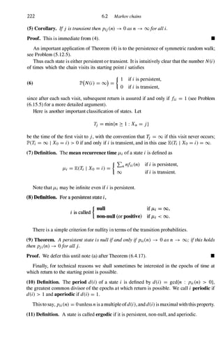
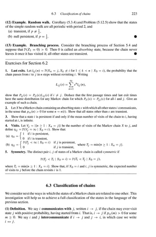
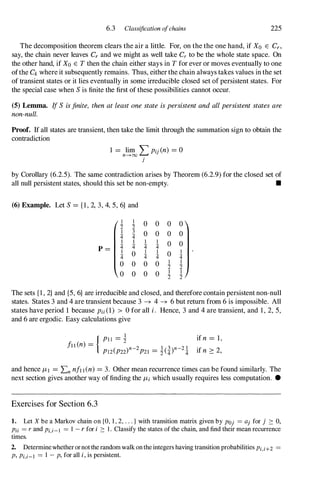
![226 6.3 Marlwv chains
3. Classify the states of the Markov chains with transition matrices
(1 -:;2P 2p 0 )
(a) 1 - 2p P ,
2p 1 - 2p
(b)
( 0 P :;
0 1 -
�P ).
I �P
I :P
I - p
In each case, calculate Pij (n) and the mean recurrence times of the states.
4. A particle performs a random walk on the vertices of a cube. At each step it remains where it is
with probability i, or moves to one of its neighbouring vertices each having probability i. Let v and
w be two diametrically opposite vertices. If the walk starts at v, find:
(a) the mean number of steps until its first return to v ,
(b) the mean number of steps until its first visit to w,
(c) the mean number of visits to w before its first return to v .
5. Visits. With the notation of Exercise (6.2.4), show that
(a) if i -+ j and i is persistent, then TJij = TJji = 1,
(b) TJij = 1 if and only if lP'(T; < 00 I Xo = i) = IP'(Tj < 00 I Xo = j) = l.
6. First passages. Let TA = min{n 2: 0 : Xn E A } , where X i s a Markov chain and A i s a subset
of the state space S, and let TJj = IP'(TA < 00 I Xo = j). Show that
{I if j E A,
TJj = L PjkTJk if j rf. A .
keS
Show further that ifx = (Xj : j E S) is any non-negative solution of these equations then Xj 2: TJj for
all j .
7. Mean first passage. In the notation of Exercise (6), let Pj = E(TA I Xo = j ) . Show that
Pj =
{�+ L PjkPk
keS
if j E A,
if j rf. A,
and that if x = (Xj : j E S) is any non-negative solution of these equations then Xj 2: Pj for all j .
8. Let X be an irreducible Markov chain and let A be a subset of the state space. Let Sr and Tr
be the successive times at which the chain enters A and visits A respectively. Are the sequences
{XSr : r 2: I}, {XTr : r 2: I} Markov chains? What can be said about the times at which the chain
exits A?
9. (a) Show that for each pair i, j ofstates ofan irreducible aperiodic chain, there exists N = N(i, j)
such that Pij (r) > 0 for all r 2: N.
(b) Show that there exists a function f such that, ifP is the transition matrix ofanirreducible aperiodic
Markov chain with n states, then Pij (r) > 0 for all states i, j, and all r 2: f(n).
(c) Show further that f(4) 2: 6 and fen) 2: (n - 1)(n - 2).
[Hint: The postage stamp lemma asserts that, for a, b coprime, the smallest n such that all integers
strictly exceeding n have the form aa + fJb for some integers a, fJ 2: 0 is (a - l)(b - 1 ).]
10. An urn initially contains n green balls and n + 2 red balls. A ball is picked at random: if it is
green then a red ball is also removed and both are discarded; if it is red then it is replaced together](https://image.slidesharecdn.com/grimmettstirzaker-probabilityandrandomprocessesthirded2001-220507085451-bb31ac14/85/Grimmett-Stirzaker-Probability-and-Random-Processes-Third-Ed-2001-pdf-237-320.jpg)
![6.4 Stationary distributions and the limit theorem 227
with an extra red and an extra green ball. This is repeated until there are no green balls in the urn.
Show that the probability the process terminates is 1/(n + 1).
Now reverse the rules: ifthe ball is green, it is replaced together with an extra green and an extra
red ball; if it is red it is discarded along with a green ball. Show that the expected number of iterations
until no green balls remain is L.-}=1(2j + 1) = n(n + 2). [Thus, a minor perturbation of a simple
symmetric random walk can be non-null persistent, whereas the original is null persistent.]
6.4 Stationary distributions and the limit theorem
How does a Markov chain Xn behave after a long time n has elapsed? The sequence {Xn}
cannot generally, of course, converge to some particular state s since it enjoys the inherent
random fluctuation which is specified by the transition matrix. However, we might hold out
some hope that the distributionof Xn settles down. Indeed, subject to certain conditions this
turns out to be the case. The classical study of limiting distributions proceeds by algebraic
manipulation of the generating functions of Theorem (6.2.3); we shall avoid this here, con
tenting ourselves for the moment with results which are not quite the best possible but which
have attractive probabilistic proofs. This section is in two parts, dealing respectively with
stationary distributions and limit theorems.
(A) Stationary distributions. We shall see that the existence of a limiting distribution for
Xn, as n--+ 00, is closely bound up with the existence of so-called 'stationary distributions'.
(1) Definition. The vector'IC is called a stationary distribution ofthe chain if 'IC has entries
(1f) : j E S) such that:
(a) 1Cj ?; 0 for all j, and L} 1C} = 1,
(b) 'IC = 'ICP, which is to say that 1C} = Li 1ft Pi} for all j.
Such a distribution is called stationary for the following reason. Iterate (1b) to obtain
'lCP
2
= (1fP)P = 'lCP = 1f, and so
(2) 1fp
n
= 1f for all n 2: O.
Now use Lemma (6.1 .8) to see that if Xo has distribution 1f then Xn has distribution 1f for all
n,showing that the distribution of Xn is 'stationary' as time passes; in such a case, of course,
1f is also the limiting distribution of Xn as n--+ 00.
Followingthe discussion afterthe decomposition theorem (6.3.4), we shall assume hence
forththatthe chainis irreducible and shall investigatetheexistence ofstationary distributions.
No assumption of aperiodicity is required at this stage.
(3) Theorem. An irreducible chain has a stationarydistribution 'IC ifandonlyifall thestates
are non-null persistent; in this case, 1t is the unique stationary distribution and is given by
1fi = fJ,i1for each i E S, "'where fJ,i is the mean recurrence time oli.
Stationary distributions 'IC satisfy 'IC = 'IC P. We may display a root x ofthe matrix equation
x = xP explicitly as follows, whenever the chain is irreducible and persistent. Fix a state k
and let Pi (k)be the mean number of visits of the chain to the state i between two successive](https://image.slidesharecdn.com/grimmettstirzaker-probabilityandrandomprocessesthirded2001-220507085451-bb31ac14/85/Grimmett-Stirzaker-Probability-and-Random-Processes-Third-Ed-2001-pdf-238-320.jpg)
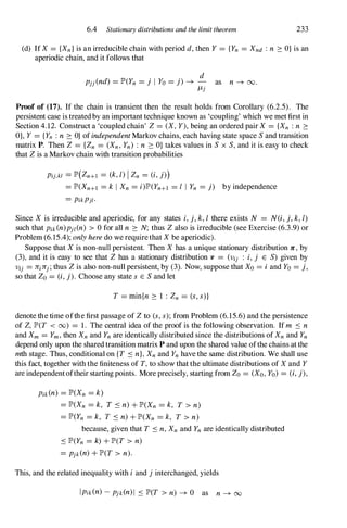

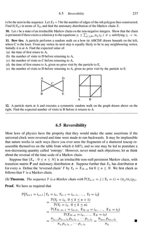
![6.6 Chains withfinitely many states
its 'Jordan canonical form' P =B-1MB where
o
o
(�1
:2
M = 0 0 J3
. . .
. . . )
241
and J1,J2, . . . are square matrices given as follows. Let )'1 , .1..2, . . . , Am be the distinct
eigenvalues of P and let ki be the multiplicity of Ai. Then
J' = O � Ii � ]
is a ki x ki matrix with each diagonal term Ai, each superdiagonal term 1, and all other terms
O. Once again we have that pn =B-1MnB, where Mn has quite a simple form (see Cox and
Miller (1965, p. 1 18 etseq.)formore details).
(2) Example. Inbreeding. Consider the genetic model described in Example (6.1.1 1c) and
suppose that C1 can take the values Aor aon each of two homologous chromosomes. Then
the possible types of individuals can be denoted by
AA, Aa (= aA), aa,
and mating between types is denoted by
AA x AA, AA x Aa, and so on.
As describedin Example (6.1 . 1 1c), meiosis causes the offspring'schromosomes to be selected
randomly from each parent; in the simplest case (since there are two choices for each of two
places) each outcome has probability i. Thus forthe offspring of AA x Aathe fourpossible
outcomes are
AA, Aa, AA, Aa
and lP'(AA) =IP'(Aa)= !. For the cross Aa x Aa,
IP'(AA) =lP'(aa)= !1P'(Aa) = i.
Clearly the offspring of AA x AAcan only be AA,and those ofaa x aacan only be aa.
We nowconstructa Markov chainby mating an individual with itself, then crossing a single
resulting offspring with itself, and so on. (This scheme is possible with plants.) The genetic
types ofthis sequence ofindividuals constitute aMarkovchain with three states, AA,Aa,aa.
In view ofthe above discussion, the transition matrix is
p= (i i D
and the reader may verify that
P' = (! _�)'+1 o 0)
o !
2
o 1
as n � 00.
Thus, ultimately, inbreeding produces a pure (AAor aa)line for which all subsequent off
spring have the same type. In like manner one can consider the progress of many different
breeding schemes which include breeding withrejection ofunfavourablegenes, back-crossing
to encourage desirable genes, and so on. •](https://image.slidesharecdn.com/grimmettstirzaker-probabilityandrandomprocessesthirded2001-220507085451-bb31ac14/85/Grimmett-Stirzaker-Probability-and-Random-Processes-Third-Ed-2001-pdf-252-320.jpg)
![242 6.6 Markov chains
Exercises for Section 6.6
The first two exercises provide proofs that a Markov chain with finitely many states has a stationary
distribution.
1. The Markov-Kakutani theorem asserts that, for any convex compact subset C of ]Rn and any
linear continuous mapping T of C into C, T has a fixed point (in the sense that T(x) = x for some
x E C). Use this to prove that a finite stochastic matrix has a non-negative non-zero left eigenvector
corresponding to the eigenvalue 1 .
2. Let T be a m x n matrix and let v E ]Rn. Farkas's theorem asserts that exactly one of the following
holds:
(i) there exists x E ]Rm such that x � 0 and xT = v,
(ii) there exists y E ]Rn such that yv
'
< 0 and Ty' � O.
Use this to prove that a finite stochastic matrix has a non-negative non-zero left eigenvector corre
sponding to the eigenvalue 1 .
3. Arbitrage. Suppose you are betting on a race with m possible outcomes. There are n bookmakers,
and a unit stake with the ith bookmaker yields tij if the jth outcome of the race occurs. A vector
x = (Xl , x2, . . . , xn), where Xr E (-00, 00) is your stake with the rth bookmaker, is called a betting
scheme. Show that exactly one of (a) and (b) holds:
(a) there exists a probability mass function p = (PI , P2, . . . , Pm) such that 2:j=1 tijPj = 0 for all
values of i,
(b) there exists a betting scheme x for which you surely win, that is, 2:1=1 Xitij > 0 for all j .
4. Let X be a Markov chain with state space S = {I, 2, 3} and transition matrix
where 0 < P < 1 . Prove that
(1 - P
p = 0
P
P
I - p
o
pn = (:�� :�� :��)
a2n a3n aln
where aln + wa2n + w2a3n = ( 1 - P + pw)n, w being a complex cube root of 1 .
5. Let P be the transition matrix of a Markov chain with finite state space. Let 1 be the identity
matrix, U the l S I x l S I matrix with all entries unity, and 1 the row l S I-vector with all entries unity.
Let Jr be a non-negative vector with 2:i Jri = 1 . Show that JrP = 1l" if and only if 1l" (I -P + U) = 1.
Deduce that if P is irreducible then 1l" = 1(I - P + U)- I .
6. Chess. A chess piece performs a random walk on a chessboard; at each step it is equally likely
to make any one of the available moves. What is the mean recurrence time of a comer square if the
piece is a: (a) king? (b) queen? (c) bishop? (d) knight? (e) rook?
7. Chess continued. A rook and a bishop perform independent symmetric random walks with
synchronous steps on a 4 x 4 chessboard (16 squares). If they start together at a comer, show that the
expected number of steps until they meet again at the same comer is 448/3.
8. Find the n-step transition probabilities Pij (n) for the chain X having transition matrix
P=(;3' t �).
4 12](https://image.slidesharecdn.com/grimmettstirzaker-probabilityandrandomprocessesthirded2001-220507085451-bb31ac14/85/Grimmett-Stirzaker-Probability-and-Random-Processes-Third-Ed-2001-pdf-253-320.jpg)
![6.8 Birthprocesses and the Poisson process 247
(1) Definition. A Poisson process with intensity )" is a process N == {N(t) : t 2: O} taking
values in S == to, 1, 2, . . . } such that:
(a) N(O) == 0; if s < t then N(s) :.:; N(t),
{)"h + o(h) ifm "'" 1,
(b) lP'(N(t + h) == n + m I N(t) "'" n) == o(h) ifm > 1,
l - Ah + o(h) ifm == O,
(c) if s < t. the number N(t) - N(s) of emissions in the interval (s, t] is independent of
the times of emissions during [0. s}.
We speakofN(t)as the numberof 'arrivals' or 'occurrences' or 'events', orin this example
'emissions', ofthe process by time t. The process Nis called a 'counting process' and is one
of the simplest examples of continuous-time Markov chains. We shall consider the general
theory of such processes in the next section; here we study special properties of Poisson
processes and their generalizations.
We are interested first in the distribution of N(t).
(2) Theorem. N(t) hasthePoissondistributionwithparameterAt; thatistosay,
(At)j
lP'(N(t) = j) = _.,_e-At,
J .
j = 0, 1, 2, . . . .
Proof. Condition N(t+ h)on N(t)to obtain
lP'(N(t+ h) = j) = LlP'(N(t) = i)lP'(N(t+ h) = j I N(t) = i)
i
= LlP'(N(t) = i)lP'((j -i)arrivals in (t,t+ hJ)
= lP'(N(t) = j - 1)lP'(one arrival) + lP'(N(t) = j)lP'(no arrivals) + o(h).
Thus Pj(t) = lP'(N(t) = j) satisfies
Pj(t+ h) = 'AhPj-l(t)+ (1 -'Ah)pj(t)+ o(h) if j =1= 0,
po(t+ h) = (1 -)"h)po(t)+ o(h).
Subtract pj(t) from each side of the first of these equations, divide by h, and let h + 0 to
obtain
(3)
likewise
(4)
The boundary condition is
(5)
pb(t) = -'Apo(t).
{ 1 if j = 0,
Pj(O) = 8jo=
0 if j =1= O.](https://image.slidesharecdn.com/grimmettstirzaker-probabilityandrandomprocessesthirded2001-220507085451-bb31ac14/85/Grimmett-Stirzaker-Probability-and-Random-Processes-Third-Ed-2001-pdf-258-320.jpg)
![N(t)
5
4
3
2
I
6.8 Birthprocesses and the Poissonprocess
•
•
•
.....--...:
•
Figure 6. 1 . A typical realization of a Poisson process N(t).
249
There is an important generalization of this result to arbitrary continuous-time Markov
chains with countable state space. We shall investigate this in the next section.
Proof. First consider Xl :
lP'(XI > t) = lP'(N(t) = 0) = e-At
and so Xl is exponentially distributed. Now, conditional on XI ,
lP'(X2 > t I Xl = tl) = lP'(no arrival in (tl,tl + t]IXl = tl).
The event {XI = tl} relates to arrivals during the time interval [0,tll, whereas the event
{no arrival in (tl,tl + t]) relates to arrivals after time tl. These events are independent, by
(Ic), and therefore
lP'(X2 > tIXl = tl) = lP'(no arrival in (tl,tl + tJ) = e-At.
Thus X2 is independent of Xl,and has the same distribution. Similarly,
lP'(Xn+l > tIXl = tl,··· , Xn = tn) = lP'(no arrival in (T, T + tJ)
where T = tl + t2 + . . . + tn,and the claim ofthe theorem follows by induction on n. •
It is not difficult to see that the process N, constructed by (9) from a sequence Xl , X2, . . . ,
is a Poisson process if and only if the Xi are independent identically distributed exponential
variables (exercise: use the lack-of-memory property of Problem (4. 14.5» . If the Xi form
such a sequence, it is a simple matter to deduce the distribution of N(t) directly, as follows.
In this case, Tn = "L7 Xi is r(A, n) and N(t) is specified by the useful remark that
N(t) :::: j if and only if Tj S t.](https://image.slidesharecdn.com/grimmettstirzaker-probabilityandrandomprocessesthirded2001-220507085451-bb31ac14/85/Grimmett-Stirzaker-Probability-and-Random-Processes-Third-Ed-2001-pdf-260-320.jpg)
![252 6.8 Markov chains
There may seem something wrong here, because the condition
(17) LPi}(t) = 1
}
in conjunction with the result of (16) would constrain {Pi}(t)}to be the uniquesolution ofthe
backward system which is a proper distribution. The point is that (17)may fail to hold. A
problem arises when the birth rates An increase sufficiently quickly with nthat the process N
may pass through all (finite) states in bounded time, and we say that explosionoccurs if this
happens with a strictly positive probability. Let Too = limn--->oo Tn be the limit of the arrival
times of the process.
(18) Definition. We call the process N honest if JP>(T00 = 00) = 1 for all t,and dishonest
otherwise.
Equation (17) is equivalentto JP>(Too > t) = 1, whence (17) holds forall tifandonly if N
is honest.
(19) Theorem. TheprocessN ishonestifandonlyifLn A;;1 = 00.
This beautiful theorem asserts that if the birth rates are small enough then N(t)is almost
surely finite, but if they are sufficiently large that LA;;1 converges then births occur so
frequently that there is positive probability of infinitely many births occurring in a finite
interval of time; thus N(t) may take the value +00 instead of a non-negative integer. Think
of the deficit 1 - L} Pi}(t) as the probability JP>(T00 � t) of escaping to infinity by time t,
starting from i.
Theorem (19) is a immediate consequence ofthe following lemma.
(20) Lemma. LetXI,X2,... beindependentrandomvariables, Xnhavingtheexponential
distributionwithparameterAn-I,andletToo = Ln Xn. Wehavethat
Proof. We have by equation (5.6. 13) that
ifLn A;;I = 00,
ifLn A;;I < 00.
(00 ) 00 1
lE(Too) = lE LXn = L - .
An-I
n=l n=1
If Ln A;;I < 00 then lE(Too) < 00, whence JP>(Too = 00) = O.
In order to study the atom of Too at 00 we work with the bounded random variable e-Too,
defined as the limit as n -+ 00 of e-Tn. By monotone convergence (5.6.12),
lE(e-Too) = lEQ]e-xn) = J�oo lEQje-xn)
N
= lim n lE(e-xn)
N--->oo n=1
by independence
= lim n
N
__
1 ----;- = {n
OO(l +A;;-21)}-1
N--->oo 1 + A-1
n=l n-I n=1](https://image.slidesharecdn.com/grimmettstirzaker-probabilityandrandomprocessesthirded2001-220507085451-bb31ac14/85/Grimmett-Stirzaker-Probability-and-Random-Processes-Third-Ed-2001-pdf-263-320.jpg)
![254 6.8 Markov chains
Now, the process is temporally homogeneous, and A is defined in terms of {N(s) : s > T};it
follows that the (conditional) probability of A depends only on the value of N(T),which is
to say that
lP'(A IN(T) = i, T= T(B)) = lP'(A IN(T) = i)
and (22) follows.
To obtain (22) for more general events B than that given above requires a small spot of
measure theory. For those readers who want to see this, we note that, for general B,
lP'(A IN(T) = i, B) = lE(IA IN(T) = i, B)
= lE{lE(IA IN(T) = i, B, H) IN(T) = i, B}
where H = {N(s) : s ::::: T}. The inner expectation equals lP'(A I N(T) = i),by the argument
above, and the claim follows. •
We used two properties of birth processes in our proof of the strong Markov property:
temporal homogeneity and the weak Markov property. The strong Markov property plays an
important role in the study of continuous-time Markov chains and processes, and we shall
encounter it in a more general form later. When applied to a birth process N,it implies that
the new process N',defined by N'(t) = N(t+ T)-N(T),t 2: 0, conditional on {N(T) = i}
is also a birth process, whenever T is a stopping time for N; it is easily seen that this new
birth process has intensities Ai, Ai+1 , . . . . In the case of the Poisson process, we have that
N'(t) = N(t+ T) -N(T)is a Poisson process also.
(23) Example. A Poisson process N is said to have 'stationary independent increments',
since: (a) the distribution of N(t) - N(s) depends only on t - s, and (b) the increments
{N(ti) - N(Si) : i = 1, 2, ... ,n} are independent if Sl ::::: t1 ::::: S2 ::::: t2 ::::: ... ::::: tn. this
property is nearly a characterization ofthe Poissonprocess. Suppose thatM= {M(t) :t 2: O}
is a non-decreasingright-continuousinteger-valuedprocess with M(0) = 0, having stationary
independent increments, and with the extra property that Mhas only jump discontinuities of
size 1. Note first that, for u,v 2: 0,
lEM(u + v) = lEM(u) + lE[M(u+ v) -M(u)] = lEM(u) + lEM(v)
by the assumption of stationary increments. Now lEM(u)is non-decreasing in u,so that there
exists A such that
(23) lEM(u) = AU, u 2: O.
Let T = sup{t : M(t) = O} be the time of the first jump of M. We have from the right
continuity of Mthat M(T) = 1 (almost surely), so that Tis a stopping time for M. Now
(24) lEM(s) = lE{lE(M(s) I T)}.
Certainly lE(M(s) I T) = 0 if s < T, and for s 2: t
lE(M(s) IT = t) = lE(M(t) I T = t) + lE(M(s) -M(t) IT= t)
= 1 +lE(M(s) -M(t) IM(t) = 1, M(u) = O for u < v)
= 1 + lEM(s-t)](https://image.slidesharecdn.com/grimmettstirzaker-probabilityandrandomprocessesthirded2001-220507085451-bb31ac14/85/Grimmett-Stirzaker-Probability-and-Random-Processes-Third-Ed-2001-pdf-265-320.jpg)
![6.8 Birthprocesses and the Poissonprocess 255
by the assumption ofstationary independentincrements. We substitute this into (24)to obtain
lEM(s) = los[1 + lEM(s - t)] dF(t)
where F is the distribution function of T. Now lEM(s) = AS for all s, so that
(25) AS = F(s) + A los(s - t) dF(t),
an integral equation for the unknown function F. One of the standard ways of solving such
an equation is to use Laplace transforms. We leave it as an exerciseto deduce from (25) that
F(t) = 1 - e-At, t 2: 0, so that T has the exponential distribution. An argument similar to
that used for Theorem (10) now shows that the 'inter-jump' times of Mare independent and
have the exponential distribution. Hence Mis a Poisson process with intensity A. •
Exercises for Section 6.8
1. Superposition. Flies and wasps land on your dinner plate in the manner of independent Poisson
processes with respective intensities A and /-L. Show that the arrivals of flying objects form a Poisson
process with intensity A + /-L.
2. Thinning. Insects land in the soup in the manner of a Poisson process with intensity A, and each
such insect is green with probability p, independently of the colours of all other insects. Show that
the arrivals of green insects form a Poisson process with intensity Ap.
3. Let Tn be the time of the nth arrival in a Poisson process N with intensity A, and define the excess
lifetime process E(t) = TN(t)+l - t, being the time one must wait subsequent to t before the next
arrival. Show by conditioning on Tl that
lP' (E(t) > x) = e-A(t+x) + fot
lP' (E(t - u) > x)Ae-AU duo
Solve this integral equation in order to find the distribution function of E(t). Explain your conclusion.
4. Let B be a simple birth process (6.8. l Ib) with B(O) = I; the birth rates are An = nA. Write
down the forward system of equations for the process and deduce that
Show also that IE(B(t» = IeAt and var(B(t» = Ie2At(1 - e-At).
k ?:. I.
5. Let B be a process of simple birth with immigration (6.8. l Ic) with parameters A and v , and
with B(O) = 0; the birth rates are An = nA + V . Write down the sequence of differential-difference
equations for Pn(t) = lP'(B(t) = n). Without solving these equations, use them to show that met) =
IE(B(t» satisfies m'(t) = Am(t) + v, and solve for met).
6. Let N be a birth process with intensities AO, AI, . . . , and let N(0) = O. Show that Pn(t) =
lP'(N(t) = n) is given by
1
n n A'
Pn(t) = - LAie-Ait II __
J -
An ' 0 . 0 A; - Ai
provided that Ai =f. Aj whenever i =f. j .
1= J= J
j#i](https://image.slidesharecdn.com/grimmettstirzaker-probabilityandrandomprocessesthirded2001-220507085451-bb31ac14/85/Grimmett-Stirzaker-Probability-and-Random-Processes-Third-Ed-2001-pdf-266-320.jpg)
![6.9 Continuous-time Markov chains 257
Proof. Part (a) is obvious.
(b) With 1 a row vector ofones, we have that
(Ptl')i =�Pij(t) =lP{l){X(t) =j} IX(O) =i) = 1 .
] ]
(c) Using the Markov property,
Pij(S +t) =lP'(X(s+f) =j IX(O) =i)
=�)P'(X(s+f) =j IX(s) =k, X(O) =i)lP'(X(s) =kIX(O) =i)
k
=LPik(S)Pkj(f) as for Theorem (6.1.7). •
k
As before, the evolution of X(f) is specified by the stochastic semigroup {Pt} and the
distribution of X(0). Most questions about Xcan be rephrased in terms ofthese matrices and
their properties.
Many readers will notbe very concernedwith thegeneral theory oftheseprocesses, butwill
be much more interested in specific examples and their stationary distributions. Therefore,
we present only a broad outline of the theory in the remaining part of this section and hope
that it is sufficient for most applications. Technical conditions are usually omitted, with the
consequencethatsomeoffhestafementswhichfollowarefalseingeneral;such statements are
marked with an asterisk. Indications of how to fill in the details are given in the next section.
We shall always suppose that the transition probabilities are continuous.
(4) Definition. The semigroup {Pt} is called standard if Pt -+ I as f + 0, which is to say
that Pii(t) -+ 1 and Pij(f) -+ 0 for i =1= j as f + O.
Note that the semigroup is standard if and only ifits elements Pij(f)are continuous func
tionsoff. In orderto seethis, observe thatPij(f)iscontinuous forallfwheneverthesemigroup
is standard; we just use the Chapman-Kolmogorov equations (3c) (see Problem (6.15.14» .
Henceforth we consider only Markov chains with standard semigroups oftransition probabil
ities.
Suppose that the chain is in state X(t) = i at time f. Various things may happen in the
small time interval (t,f+h):
(a) nothing may happen, with probability Pii(h)+o(h), the error term taking into account
the possibility thatthe chain moves out of iand back to i in the interval,
(b) the chain may move to a new state j with probability Pij(h) +o(h).
We are assuminghere thatthe probabilityoftwo or moretransitions in the interval (f,f+h)
is o(h); this canbeproved. Following (a) and (b), we are interested in the behaviourofPij(h)
for small h;it turns outthat Pij(h)is approximately linear in hwhen his small. That is, there
exist constants {gij : i,j E S} such that
(5) Pij (h) ::: gijh if i :f: j, pu (h) � 1 + giih.
Clearly gij � 0 for i =1= j and gii .:s 0 for all i; the matrixt G = (gij) is called the
tSome writers use the notation qi; in place of g'j , and term the resulting matrix Q the ' Q-matrix' of the
process.](https://image.slidesharecdn.com/grimmettstirzaker-probabilityandrandomprocessesthirded2001-220507085451-bb31ac14/85/Grimmett-Stirzaker-Probability-and-Random-Processes-Third-Ed-2001-pdf-268-320.jpg)
![258 6.9 Markov chains
generator of the chain and takes over the role of the transition matrix Pfor discrete-time
chains. Combine (5) with (a) and (b) above to find that, starting from X(t) = i,
(a) nothing happens during (t,t+h)with probability 1 +giih+o(h),
(b) the chainjumps to state j (# i)with probability gijh+o(h).
One may expect that LjPij(t)= 1, and so
leading to the equation
(6*)
j j
Lgij = 0 for all i, or GI' = 0',
j
where 1 and 0 are row vectors of ones and zeros. Treat (6) with care; there are some chains
for which it fails to hold.
(7) Example. Birth process (6.8.11). From the definition ofthis process, it is clear that
Thus
gii = -Ai, gi,i+l = Ai, gij = 0 if j < i or j > i+1 .
AO
-AI
o
0
Al
-A2
0 0
)
0 0 . . .
A2 0
Relation (5) is usually written as
(8)
. 1
G
hm -(Ph - I) = ,
htOh
•
and amounts to saying that Pt is differentiable at t = O. It is clear that G can be found from
knowledge of the Pt. The converse also is usually true. We argueroughly as follows. Suppose
that X(0) = i,and condition X(t+h) on X(t) to find that
giving that
Pij(t+h) = LPik(t)Pkj(h)
k
c::: Pij(t)(1+gjjh)+ L Pik(t)gkjh by (5)
k:kf.j
= Pij(t)+hLPik(t)gkj,
k
1
h [Pij(t+h)-Pij(t)] c::: LPik(t)gkj = (PtG)ij.
k
Let h ,J, 0 to obtain the forward equations. We write P;for the matrix with entries P;j(t).](https://image.slidesharecdn.com/grimmettstirzaker-probabilityandrandomprocessesthirded2001-220507085451-bb31ac14/85/Grimmett-Stirzaker-Probability-and-Random-Processes-Third-Ed-2001-pdf-269-320.jpg)
![6.9 Continuous-time Markov chains
(9*) Forward equations. We have thatp;: = PtG, which is to say that
P�j(t) =: LPik(t)gkj forall i, j € S.
k
259
A similar argument, by conditioning X(t + h)on X(h),yields the backward equations.
(10*) Backward equations. W
e have that P� =: GPt, which is to say that
p�/t) =: LgikPkj(t) joraU i, j E S.
k
These equations are general forms of equations (6.8.12)and (6.8.13)and relate {Pt} to G.
Subject to the boundary condition Po = I, they often have a unique solution given by the
infinite sum
(11*)
00 n
L t n
Pt = -G
n!
n=O
of powers of matrices (remember that GO= I). Equation (11)is deducible from (9) or (10)in
very much the same way as we might show thatthe function ofthe single variable pet) = egt
solves the differential equation p
'
(t) = gp (t). The representation (1 1 ) for Pt is very useful
and is usually written as
(12*) Pt = etG or Pt = exp(tG).
where eAis the natural abbreviation for .E�o(l/n!)Anwhenever Ais a square matrix.
So, subjectto certaintechnicalconditions, acontinuous-timechain has ageneratorGwhich
specifies the transition probabilities. Several examples ofsuch generators are given in Section
6.1 1 . In the last section we saw that a Poisson process (this is Example (7) with Ai = A for
all i 2: 0) can be described in terms of its interarrival times; an equivalent remark holds here.
Suppose that Xes) = i. The future development of Xes + t), for t 2: 0, goes roughly as
follows. Let U = inf{t 2: 0 : X(s+ t) =f. i } be the further time until the chain changes its
state; Uis called a 'holding time'.
(13*) Claim. The random variable U is exponentially distributed withparameter -gil-
Thus the exponential distribution plays a central role in the theory ofMarkov processes.
Sketch proof. Thedistribution ofUhasthe 'lackofmemory' property (see Problem (4.14.5»
because
lP'(U > x+ y I U > x) = lP'(U > x+ y IX(t + x) = i)
= lP'(U > y) if x,y 2: 0
by the Markov property and the homogeneity of the chain. It follows that the distribution
function Fu ofUsatisfies 1-Fu(x+ y) = [1-Fu(x)][l-Fu(y)], and so 1-Fu(x) = e-J..x
where A = F&(O) = -gii. •
Therefore, if Xes) = i,the chain remains in state i for an exponentially distributed time
U,after which itjumps to some other state j.](https://image.slidesharecdn.com/grimmettstirzaker-probabilityandrandomprocessesthirded2001-220507085451-bb31ac14/85/Grimmett-Stirzaker-Probability-and-Random-Processes-Third-Ed-2001-pdf-270-320.jpg)
![260 6.9 Markov chains
(14*) Claim. The probability that the chainjumps to j (::p i) is -Sij/Su,
Sketch proof. Roughly speaking, suppose that x < U S x + hand suppose that the chain
jumps only once in (x, x + hJ. Then
JP'O
.
I " ) Pij(h) gij
umps to ] ItJumps � � - -
1 - Pii(h) gii as h ,J,O. •
(15) Example. Consider a two-state chain Xwith S = {l, 2}; Xjumps between 1 and 2 as
time passes. There are two equivalent ways of describing the chain, depending on whether
we specify G or we specify the holding times:
(-a a )
(a) Xhas generator G =
fJ -fJ ;
(b) if the chain is in state 1 (or 2), then it stays in this state for a length of time which is
exponentially distributed with parameter a(or fJ)beforejumping to 2 (or 1 ).
The forward equations (9), P; = PtG, take the form
p�I (t) = -apll(t)+ fJpn{t)
and are easily solved to find the transition probabilities ofthe chain (exercise). •
We move on to the classification ofstates; this is not such a chore as it was fordiscrete-time
chains. It turns out that for any pair i, j of states
(16) either Pij(t) = 0 for all t > 0, or Pij(t) > 0 for all t > 0,
and this leads to a definition of irreducibility.
(17) Definition. The chain is called irreducible if for any pair i, j of states we have that
Pij(t) > 0 for some t.
Any time t > 0 will suffice in (17), because of (16). The birth process is notirreducible,
since it is non-decreasing. See Problem (6.15.15) for a condition for irreducibility in terms of
the generator G ofthe chain.
As before, the asymptotic behaviour of X(t) for large t is closely bound up with the
existence of stationary distributions. Compare their definition with Definition (6.4.1).
(18) Definition. The vecton'r is a stationary distribution ofthe chain iftr} 2:: O. Lj ;If} = 1.
and 1£ "" 1£Pt for all t 2:: O.
If X(0) has distribution /L(0) then the distribution /L(t) of X(t) is given by
(19)
If /L(0) = /L, a stationary distribution, then X(t)has distribution /L for all t. For discrete-time
chains we found stationary distributions by solving the equations Jr = JrP; the corresponding
equations Jr = JrPt for continuous-time chains may seem complicated but they amount to a
simple condition relating Jr and G.](https://image.slidesharecdn.com/grimmettstirzaker-probabilityandrandomprocessesthirded2001-220507085451-bb31ac14/85/Grimmett-Stirzaker-Probability-and-Random-Processes-Third-Ed-2001-pdf-271-320.jpg)
![6.9 Continuous-time Markov chains 265
[The full assumption of the independence of N and X is not necessary for the conclusion. It suffices
that {N(s) : s 2: t} be independent of {X(s) : s ::: t}, a property known as 'lack of anticipation' . It is
not even necessary that X be Markov; the Pasta property holds for many suitable ergodic processes.]
5. Let X be a continuous-time Markov chain with generator G satisfying gi = -gii > 0 for all i.
Let HA = inf{t 2: 0 : X (t) E A} be the hitting time of the set A of states, and let 7)j = JP'(HA < 00 I
X(0) = j) be the chance of ever reaching A from j . By using properties of the jump chain, which
you may assume to be well behaved, show that 2:k gjk7)k = 0 for j 1. A.
6. In continuation of the preceding exercise, let f-tj = E(HA I X (0) = j). Show that the vector IL
is the minimal non-negative solution of the equations
f-tj = 0 if j E A , 1 + L gjkf-tk = 0 if j 1. A .
kES
7. Let X be a continuous-time Markov chain with transition probabilities Pij (t) and define Fi
inf{t > TJ : X(t) = i} where TJ is the time of the first jump of X. Show that, if gji =f. 0, then
JP'(Fi < 00 I X (0) = i) = 1 if and only if i is persistent.
8. Let X be the simple symmetric random walk on the integers in continuous time, so that
Pi,i+1 (h) = Pi,i-I (h) = 1Ah + o(h) .
Show that the walk i s persistent. Let T be the time spent visiting m during an excursion from O. Find
the distribution of T.
9. Let i be a transient state of a continuous-time Markov chain X with X (0) = i. Show that the
total time spent in state i has an exponential distribution.
10. Let X be an asymmetric simple random walk in continuous time on the non-negative integers
with retention at 0, so that
{ Ah + o(h) if j = i + 1 , i 2: 0,
Pij (h) = . . . .
f-th + o(h) If J = I - 1 , I 2: 1 .
Suppose that X (0) = 0 and A > f-t. Show that the total time Vr spent in state r is exponentially
distributed with parameter A - f-t.
Assume now that X (0) has some general distribution with probability generating function G.
Find the expected amount of time spent at 0 in terms of G.
11. Let X = {X(t) : t 2: O} be a non-explosive irreducible Markov chain with generator G and unique
stationary distribution 1C. The mean recurrence time f-tk is defined as follows. Suppose X (0) = k,
and let U = inf{s : X (s) =f. k}. Then f-tk = E(inf{t > U : X (t) = k}). Let Z = { Zn : n 2: O} be the
imbedded 'jump chain' given by Zo = X (0) and Zn is the value of X just after its nth jump.
(a) Show that Z has stationary distribution ii satisfying
where gi = -gii, provided 2:i 7iigi < 00. When is it the case that ii = 1C?
(b) Show that tii = l/(f-tigi) if f-ti < 00, and that the mean recurrence time 11kof the state k in the
jump chain Z satisfies 11k = f-tk 2:i tiigi if the last sum is finite.
12. Let Z be an irreducible discrete-time Markov chain on a countably infinite state space S, having
transition matrix H = (hij) satisfying hii = 0 for all states i, and with stationary distribution v .
Construct a continuous-time process X on S for which Z is the imbedded chain, such that X has no
stationary distribution.](https://image.slidesharecdn.com/grimmettstirzaker-probabilityandrandomprocessesthirded2001-220507085451-bb31ac14/85/Grimmett-Stirzaker-Probability-and-Random-Processes-Third-Ed-2001-pdf-276-320.jpg)
![268 6. 1 1 Markov chains
is the generator of a uniform stochastic semigroup {Pt } given by the following calculation.
Diagonalize G to obtain G =BAB-1 where
Therefore
Pt =f::�Gn =B (f::�An)B-1
n=O n=O
=B (hg) �)B-1 since A0 =I
1
( ah(t) +fi
= a +fi fi[1 -h(t)] a[1 -h(t)])
a +fih(t)
where h(t) =e-t(a+f3). Let t � 00 to obtain
and so
P � (1 - p p
)
t 1 - p p
a
where p = a +fi
{ 1 - P
lP'(X(t) =i) �
P
if i = 1,
if i =2,
irrespective ofthe initial distribution of X(0). This shows that 1C = (1 - p, p) is the limiting
distribution. Check that 1CG = O. The method of Example (6.9. 15) provides an alternative
and easier route to these results. •
(13) Example. Birth process. Recall the birth process of Definition (6.8. 1 1), and suppose
that Ai > 0 for all i. The process is uniform if and only if supd-gii} =SUpdAd < 00, and
this is a sufficient conditionforthe forward andbackwardequations to have unique solutions.
We saw in Section 6.8 that the weaker condition LiAiI =00 is necessary and sufficient for
this to hold. •
6.11 Birth-death processes and imbedding
A birth process is a non-decreasing Markov chain for which the probability of moving from
state nto state n+1 in the time interval (t,t+h)is Anh+o(h). More realistic continuous-time
models for population growth incorporate death also. Suppose then that the number X(t) of
individuals alive in some population at time tevolves in the following way:
(a) Xis a Markov chain taking values in {O, 1 , 2, . . . },
(b) the infinitesimal transition probabilities are given by
(1)
(Anh+o(h)
lP'(X(t+h) =n+m/X(t) =n) = f.tnh+o(h)
o(h)
ifm = 1 ,
if m = - 1 ,
if lml > 1 ,](https://image.slidesharecdn.com/grimmettstirzaker-probabilityandrandomprocessesthirded2001-220507085451-bb31ac14/85/Grimmett-Stirzaker-Probability-and-Random-Processes-Third-Ed-2001-pdf-279-320.jpg)
 + o(u - 1) as u t I.
•
• •](https://image.slidesharecdn.com/grimmettstirzaker-probabilityandrandomprocessesthirded2001-220507085451-bb31ac14/85/Grimmett-Stirzaker-Probability-and-Random-Processes-Third-Ed-2001-pdf-284-320.jpg)
![274 6.12 Marlwv chains
Exercises for Section 6. 1 1
1. Describe the jump chain for a birth-death process with rates An and ILn .
2. Consider an immigration-death process X, being a birth-death process with birth rates An = A
and death rates ILn = nIL. Find the transition matrix of the jump chain Z, and show that it has as
stationary distribution
Jrn = _
1_ (1+ �) pne-p
2(n!) p
where p = AIIL. Explain why this differs from the stationary distribution of X.
3. Consider the birth-death process X with An = nA and ILn = nIL for all n 2: O. Suppose X (0) = 1
and let I) (t) = lP'(X (t) = 0). Show that I) satisfies the differential equation
I)'(t) + (A + IL)I) (t) = IL + AI) (t)
2
.
Hence find I) (t), and calculate lP'(X (t) = 0 I X (u) = 0) for 0 < t < u.
4. For the birth-death process of the previous exercise with A < IL, show that the distribution of
X (t), conditional on the event {X(t) > OJ, converges as t ---+ 00 to a geometric distribution.
5. Let X be a birth-death process with An = nA and ILn = nIL, and suppose X (O) = 1 . Show that
the time T at which X (t) first takes the value 0 satisfies
{� log (�) it A < IL,
E(T I T < 00) = �
(
IL � A
)
- log -- it A > IL.
IL A - IL
What happens when A = IL?
6. Let X be the birth-death process of Exercise (5) with A =I- IL, and let Vr (t) be the total amount
of time the process has spent in state r 2: 0, up to time t. Find the distribution of VI (00) and the
generating function I:r srE(Vr (t» . Hence show in two ways that E(VI (00» = [max{A, IL}]- I
.
Show further that E(Vr (oo» = Ar- I
r- l
[max{A , IL}rr .
7. Repeat the calculations of Exercise (6) in the case A = IL.
6.12 Special processes
There are many more general formulations of the processes which we modelled in Sections
6.8 and 6.1 1 . Here is a very small selection of some ofthem, with some details ofthe areas
in which they have been found useful.
(1) Non-homogeneous chains. We may relax the assumption thatthe transitionprobabilities
Pi} (s, t) = JP>(X (t) = j I X(s) = i) satisfy the homogeneity condition Pi} (s,t) = Pi} (0, t -
s). This leads to some very difficult problems. We may make some progress in the special
case when X is the simple birth-death process ofthe previous section, forwhich An = nA and
f-tn = nf-t. The parameters A and f-t are now assumed to be non-constantfunctions oft. (Mter
all, most populations have birth and death rates which vary from season to season.) It is easy
to checkthat the forward equation (6. 1 1 . 1 1) remains unchanged:
a G a G
at = [A(t)S - f-t(t)](s - 1)a;-.](https://image.slidesharecdn.com/grimmettstirzaker-probabilityandrandomprocessesthirded2001-220507085451-bb31ac14/85/Grimmett-Stirzaker-Probability-and-Random-Processes-Third-Ed-2001-pdf-285-320.jpg)
![The solution is
where I =X(0)and
6.12 Specialprocesses
er(t) t
[
_I]t
G(s,t) = 1 + (s_
1 -fo A(u)er(u)dU)
r(t) =fot[Jt(u)-A(U)]duo
275
The extinction probability lP'(X(t) =0)is the coefficient of sOin G(s,t), and it is left as an
exercisefor the reader to prove the next result.
(2) Theorem. lP'(X(t) =0) � 1 ifandonly if
fo
T
Jt(u)er(u)du � 00 as T � 00 . •
(3) A bivariate branching process. We advertised the branching process as a feasible model
for the growth of cell populations; we should also note one of its inadequacies in this role.
Even the age-dependent process cannot meet the main objection, which is that the time of
division of a cell may depend rather more on the sizeofthe cell than on its age. So here is a
model for the growth and degradation of long-chain polymerst.
A population comprises particles. Let N(t)be the number ofparticles present at time t,
and suppose that N(O) = 1 . We suppose that the N(t) particles are partitioned into W(t)
groups of size NI,N2,... ,Nw such that the particles in each group are aggregated into a
unitcell. Think of the cells as a collection of W(t) polymers, containing NI,N2,... ,Nw
particles respectively. As time progresses each cell grows and divides. We suppose that each
cell can accumulate one particle from outside the system with probability Ah +o(h) in the
time interval (t,t +h). As cells become larger they are more likely to divide. We assume
that the probability that a cell of size N divides into two cells of sizes M and N - M, for
some 0 < M < N, during the interval (t,t+h), is Jt(N- l)h +o(h). The assumption that
the probability of division is a linearfunction of the cell size N is reasonable for polymer
degradationsince theparticles are strungtogetherin aline and any ofthe N-1 'links' between
pairs ofparticles may sever. At time tthereare N(t)particles and W(t)cells, and the process
is said to be in state X(t) = (N(t),W(t». During the interval (t,t+h) various transitions
for X(t) are possible. Either some cell grows or some cell divides, or more than one such
event occurs. The probability that some cell grows is AWh +o(h) since there are Wchances
ofthis happening; the probability of a division is
Jt(NI +...+Nw - W)h +o(h) =Jt(N- W)h +o(h)
since there are N- Wlinks in all; the probability of more than one such occurrence is o(h).
Putting this information together results in a Markov chain X(t) = (N(t), W(t» with state
space {I, 2, ...}2and transition probabilities
lP'(X(t+h) = (n,w)+E IX(t) = (n,w»)
ifE = (1,0),
Jt(n-w)h+o(h) ifE = (0, 1),
{Awh+o(h)
- 1 -[W(A -Jt)+Jtn]h+o(h) if E = (0,0),
o(h) otherwise.
tIn physical chemistry, apolymer is a chain ofmolecules, neighbouring pairs ofwhich are joined by bonds.](https://image.slidesharecdn.com/grimmettstirzaker-probabilityandrandomprocessesthirded2001-220507085451-bb31ac14/85/Grimmett-Stirzaker-Probability-and-Random-Processes-Third-Ed-2001-pdf-286-320.jpg)
![276 6.12 Markov chains
Write down the forward equations as usual to obtain that the joint generating function
satisfies the partial differential equation
aG aG aG
- = f-Lx(y- 1)- + y[)..(x- 1) -f-L(Y- 1)]
at � �
with G(x, y;0) = xy. The joint moments of N and W are easily derived from this equa
tion. More sophisticated techniques show that N(t) -+ 00, W(t) -+ 00, and N(t)/ W(t)
approaches some constant as t -+ 00.
Unfortunately, most cells in nature are irritatingly non-Markovian! •
(4) A non-linear epidemic. Consider a population of constant size N + 1, and watch the
spread of a disease about its members. Let X (t) be the number of healthy individuals at time
t and suppose that X(0) = N. We assume that if X(t) = n then the probability of a new
infection during (t, t + h) is proportional to the number of possible encounters between ill
folk and healthy folk. That is,
lP'(X (t + h) = n - 1 1 X (t) = n) = )..n(N + I - n)h + o(h).
Nobody ever gets better. In the usual way, the reader can show that
N
satisfies
G(s,t) = lE(sX(t) = L::>n
lP'(X(t) = n)
n=O
aG ( aG a2G)
at = )..(1 -s) Na:; - s as2
with G(s,0) = sN. There is no simple way ofsolving this equation, though alotofinformation
is available about approximate solutions. •
(5) Birth-death with immigration. We saw in Example (6.11.6) that populations are not
always closed and that there is sometimes a chance that a new process will be started by an
arrival from outside. This may be due to mutation (if we are counting genes), or leakage (if
we are counting neutrons), or irresponsibility (if we are counting cases of rabies).
Suppose that there is one individual in the popUlation at time zero; this individual is the
founding member of some birth-death process N with fixed but unspecified parameters. Sup
pose further that other individuals immigrate into the popUlation in the manner of a Poisson
process Iwith intensity v. Each immigrant starts a new birth-death process which is an inde
pendent identically distributed copy ofthe original process N but displaced in time according
to its time of arrival. Let To (= 0), Tl , T2, . . . be the times at which immigrants arrive, and
let Xl , X2, . . . be the interarrival times Xn = Tn - Tn-I . The total population at time t is the
aggregate of the processes generated by the I(t) + 1 immigrants up to time t. Call this total
Y(t) to obtain
I (t)
(6) Y(t) = LNi (t - 1';)
i=O](https://image.slidesharecdn.com/grimmettstirzaker-probabilityandrandomprocessesthirded2001-220507085451-bb31ac14/85/Grimmett-Stirzaker-Probability-and-Random-Processes-Third-Ed-2001-pdf-287-320.jpg)
![6.12 Specialprocesses 277
where Nt , N2, . . . are independent copies of N = No. The problem is to find how the
distribution of Y depends on the typical process N and the immigration rate v ; this is an
example of the problem of compounding discussed in Theorem (5.1.25).
First we prove an interesting result about order statistics. Remember that I is a Poisson
process and Tn = inf{t : I(t) = n} is the time ofthe nth immigration.
(7) Theorem. TheconditionaljointdistributionofTt , Tz, . . . ,Tn, conditionalontheevent
{I (t) = n}, is the same as thejoint distribution oftheorderstatistics ofafamily ofn
independentvariableswhichareuniformlydistributedon[0, t].
This is something ofa mouthful, and asserts thatifwe know that nimmigrants have arrived
by time t then their actual arrival times are indistinguishable from a collection of n points
chosen uniformly at random in the interval [0, t].
Proof. We want the conditional density function ofT = (Tl, T2, . . . , Tn) given that I (t) = n.
First note that Xt , X2, . . . , Xn are independent exponential variables with parameter v so that
Make the transformation X � T and use the change of variable formula (4.7.4) to find that
Let C C ]Rn. Then
(8)
but
(9)
and
(10)
(T C I )
lP'(I(t) =nandTE C)
lP' E I(t) = n = ,
lP'(I = n)
lP'(I(t) = n and T E C) = LlP'(I(t) = ni T = t)h(t) dt
= LlP'(I(t) = nI Tn = tn)h(t) dt
so long as tn .:s t. Substitute (10) into (9) and (9) into (8) to obtain
where
lP'(T E C I I(t) = n) = LL(t)n! t-n dt
{ I if tl < t2 < . . . < tn,
L(t) =
° otherwise.
We recognize g(t) = L(t)n! t-n from the result of Problem (4.1 4.23) as the joint density
function of the order statistics of nindependent uniform variables on [0, t]. •](https://image.slidesharecdn.com/grimmettstirzaker-probabilityandrandomprocessesthirded2001-220507085451-bb31ac14/85/Grimmett-Stirzaker-Probability-and-Random-Processes-Third-Ed-2001-pdf-288-320.jpg)
![278 6.12 Markov chains
We are now ready to describe Y(t)in terms of the constituent processes M .
(11) Theorem. If N(t) hasgeneratingfunction GN(S,t) = lE(sN(t» then thegenerating
functionG(s, t) = lE(sY(t» satisfies
Proof. Let UI, U2, . . . be a sequence of independent uniform variables on [0, t]. By (6),
where I = I(t). By independence, conditional expectation, and (7),
(12)
However,
(13)
(14)
lE(sY(t» = lE(sNo(t» lE{lE(sN1 (t-T1)+·+N/(t-T/) I I)}
= GN(S,t)lE{lE(SN1 (t-U1)+·+N/ (t-U/) I I)}
= GN(S,t)lE{lE(sN1 (t-U1» I }.
and
Substitute (13)and (14)into (12)to obtain the result. • •
(15) Branching random walk. Another characteristic of many interesting populations is
their distribution about the space that they inhabit. We introduce this spatial aspect gently,
by assuming that each individual lives at some point on the real line. (This may seem a
fair description of a sewer, river, or hedge.) Let us suppose that the evolution proceeds as
follows. After its birth, a typical individual inhabits a randomly determined spot X in � for
a random time T. After this time has elapsed it dies, leaving behind a family containing N
offspring which it distributes at points X + YI, X + Y2, . . . , X + YN where YI , Y2, . . . are
independent and identically distributed. These individuals then behave as their ancestor did,
producing the next generation offspring after random times at points X + Yi + Yij, where Yij
is the displacement of the jth offspring of the ith individual, and the Yij are independent and
identically distributed. We shall be interested in the way that living individuals are distributed
about � at some time t.
Suppose that the process begins with a single newborn individual at the point O. We require
some notation. Write GN(S)for the generating function of a typical family size N and let F
be the distribution function of a typical Y. Let Z(x,t) be the number of living individuals at
points in the interval (-00, x]at time t. We shall study the generating function
G(s;x,t) = lE(sZ(x,t» .](https://image.slidesharecdn.com/grimmettstirzaker-probabilityandrandomprocessesthirded2001-220507085451-bb31ac14/85/Grimmett-Stirzaker-Probability-and-Random-Processes-Third-Ed-2001-pdf-289-320.jpg)
![6.12 Specialprocesses 279
Let T be the lifetime of the initial individual, N its family size, and Yl, Y2, . . . , YN the
positions of its offspring. We shall condition Z on all these variables to obtain a type of
backward equation. We must be careful about the order in which we do this conditioning,
because the length of the sequence Yl, Y2, . . . depends on N. Hold your breath, and note
from Problem (4.14.29) that
Clearly
G(s;x,t) = lE{lE[lE(lE(SZ I T, N,Y) I T, N) I T]}.
{ Z(X, O) if T > t,
Z(x, t) = N .
Li=l Zi(X - Yi, t - T) If T S t,
where the processes ZI , Z2, . . . are independent copies of Z. Hence
lE(SZ I T, N,Y) =
{ G�;x,0) if T > t,
ni=l G(s; x - Yi, t - T) if T S t.
Thus, if T S t then
lE[lE(lE(SZ I T, N,Y) I T, N) I T] = lE [(I:G(s;x- y,t - T) dF(y)rIT]
= GN (i:G(s;x - y,t - T) dF(Y)).
Now breathe again. We consider here only the Markovian case when T is exponentially
distributed with some parameter J-L. Then
Substitute v = t - u inside the integral and differentiate with respect to t to obtain
aG + J-LG = J-LGN (rJO G(s;x- y,t) dF(Y)).
at J-oo
It is not immediately clear that this is useful. However, differentiate withrespectto sat s = I
to find that m(x,t) = lE(Z(x, t)) satisfies
am
1
00
- + J-Lm = J-LlE(N) m(x- y,t) dF(y)
at -00
which equation is approachable by Laplace transform techniques. Such results can easily be
generalized to higher dimensions. •
(16) Spatial growth. Here is a simple model for skin cancer. Suppose that each point (x,y)
of the two-dimensional square lattice 712 = {(x,y) : x,y = 0, ±1, ±2, . . . } is a skin cell.
There are two types of cell, called b-cells (benigncells) and m-cells (malignantcells). Each
cell lives foran exponentially distributed period oftime, parameter f3 for b-cells and parameter](https://image.slidesharecdn.com/grimmettstirzaker-probabilityandrandomprocessesthirded2001-220507085451-bb31ac14/85/Grimmett-Stirzaker-Probability-and-Random-Processes-Third-Ed-2001-pdf-290-320.jpg)
![6.13 Spatial Poissonprocesses 281
their arrival by a single assistant; each service period is a random variable which we assume
to be exponential with parameter /1 and which is independent of all other considerations. Let
X(t)be the length of the waiting line at time t(including any person being served). It is easy
to see that X is a birth-death process with parameters An = A for n :::: 0, /1n = /1 for n :::: 1 .
The server would be very unhappy indeed if the queue length X(t)were to tend to infinity as
t-+ 00, since then he or she would have very few tea breaks. It is not difficult to see that the
distribution of X(t)settles down to a limit distribution, as t -+ 00, if and only ifA < /1, which
is to say that arrivals occur more slowly than departures on average (see condition (6. 1 1.3)).
We shall consider this process in detail in Chapter 1 1, together with other more complicated
queueing models. •
Exercises for Section 6. 1 2
1. Customers entering a shop are served in the order of their arrival by the single server. They
arrive in the manner of a Poisson process with intensity A, and their service times are independent
exponentially distributed random variables with parameter /-t. By considering the jump chain, show
that the expected duration of a busy period B of the server is (/-t - A)-1 when A < /-t. (The busy
period runs from the moment a customer arrives to find the server free until the earliest subsequent
time when the server is again free.)
2. Disasters. Immigrants arrive atthe instants ofa Poisson process ofrate 1J , and each independently
founds a simple birth process of rate A. At the instants of an independent Poisson process of rate 8,
the population is annihilated. Find the probability generating function of the population X(t), given
that X(0) = o.
3. More disasters. In the framework of Exercise (2), suppose that each immigrant gives rise to a
simple birth-death process of rates A and /-t. Show that the mean population size stays bounded if and
only if 8 > A - /-t .
4. The queue MlG/oo. (See Section 1 1 . 1 .) An ftp server receives clients at the times of a Poisson
process with parameter A, beginning at time O. The ith client remains connected for a length Sj
of time, where the Si are independent identically distributed random variables, independent of the
process of arrivals. Assuming that the server has an infinite capacity, show that the number of clients
being serviced at time t has the Poisson distribution with parameter A fci[l - G (x)] dx, where G is
the common distribution function of the Sj.
6.13 Spatial Poisson processes
The Poisson process of Section 6.8 is a cornerstone of the theory of continuous-time Markov
chains. It is also a beautiful process in its own right, with rich theory and many applications.
While the process of Section 6.8 was restricted to the time axis IR+ = [0, 00), there is a useful
generalization to the Euclidean space IRd where d :::: 1.
We begin with a technicality. Recall that the essence of the Poisson process of Section 6.8
was the set of arrival times, a random countable subset of IR+. Similarly, a realization of a
Poisson process on IRd will be a countable subset nof IRd. We shall study the distribution of
Il through the number I Il n A I of its points lying in a typical subset A of IRd. Some regularity
will be assumed about such sets A, namely that there is a well defined notion of the 'volume'
of A. Specifically, we shall assume that A E fBd, where fBd denotes the Borel a-field of IRd,
being the smallest a-field containing all boxesof the form n1=1 (aj, bd. Members of fBd are
called Borelsets,and we write IA I for the volume (or Lebesgue measure) of the Borel set A.](https://image.slidesharecdn.com/grimmettstirzaker-probabilityandrandomprocessesthirded2001-220507085451-bb31ac14/85/Grimmett-Stirzaker-Probability-and-Random-Processes-Third-Ed-2001-pdf-292-320.jpg)
![282 6.13 Marlwv chains
(1) Definition. The random countable subset n of Rd is called a Poisson process with
(constant)intensity A if, for all A E 1Bd, the random variables N(A) .", III n AI satisfy:
(a) N(A) has the Poisson distribution with parameter AlAI, and
(b) if At, Al• . . . , An are disjointsets in jJd, then N(Al), N(A2). � . . , N(An) are indepen
dent random variables.
We often refer to the counting process Nas being itself a Poisson process if it satisfies (a)
and (b) above. In the case when A > 0 and IAI = 00, the number Inn AI has the Poisson
distribution with parameter 00, a statement to be interpreted as lP'(lnn AI = 00) = 1.
It is not difficult to see the equivalence of (1) and Definition (6.8.1) when d= 1. That is,
if d= 1 and Nsatisfies (1), then
(2) M(t) = N([O,t1), t 2: 0,
satisfies (6.8.1). Conversely, if M satisfies (6.8.1), one may find a process Nsatisfying (1)
such that (2) holds. Attractive features ofthe above definition include the facts that the origin
plays no special role, and that the definition may be extended to sub-regions of ]Rd as well as
to a-fields of subsets of general measure spaces.
There are many stochastic models based on the Poisson process. One-dimensional pro
cesses were used by Bateman, Erlang, Geiger, and Rutherford around 1909 in their investiga
tions of practical situations involving radioactive particles and telephone calls. Examples in
two and higher dimensions include the positions of animals in their habitat, the distribution
of stars in a galaxy or of galaxies in the universe, the locations of active sites in a chemical
reaction or ofthe weeds in your lawn, and the incidence of thunderstorms and tornadoes. Even
when a Poisson process is not a perfect description of such a system, it can provide arelatively
simple yardstick against which to measure the improvements which may be offered by more
sophisticated but often less tractable models.
Definition (1) utilizes as reference measure the Lebesgue measure on ]Rd, in the sense that
the volume of a set A is its Euclidean volume. It is useful to have a definition of a Poisson
process with other measures than Lebesgue measure, and such processes are termed 'non
homogeneous' . Replacing the Euclidean element Adxwith the element A(X)dx,we obtain
the following, in which A(A)is given by
(3) A(A) = iA(x)dx, A E :J3d.
(4) Definition. Let d � 1 and let A : Rd -+ R be a non-negative measurable function such
that A(A) < 00 for all bounded A. The random countable subset n of lR.d is called a non
homogeneous Poisson process with intensity fnnction A if, for all A E fBd, the random
variables N(A) = III n AI satisfy:
(a) N(A) has the Poisson distribution with parameter A(A), and
(b) if At, A2. " . , An are disjoint sets in /Bd, then N(Al), N(A2)• . . . , N(An) are indepen
dentrandom variables.
We call the function A(A), A E j3d, the mean measure of the process n. We have
constructed Aas the integral (3) ofthe intensity function A;one may in fact dispense altogether
with the function A, working instead with measures Awhich 'have no atoms' in the sense that
A({x}) = 0 for all xE ]Rd.](https://image.slidesharecdn.com/grimmettstirzaker-probabilityandrandomprocessesthirded2001-220507085451-bb31ac14/85/Grimmett-Stirzaker-Probability-and-Random-Processes-Third-Ed-2001-pdf-293-320.jpg)
![6.13 Spatial Poissonprocesses 283
Our first theorem states that the union of two independent Poisson processes is also a
Poisson process. A similar result is valid for the union of countably many independent
Poisson processes.
(5) Superposition theorem. LetTI'andTI" beindependentPoissonprocesseson]Rd with
respective intensityfunctionsA' andA". Theset TI = TI'U TI" isaPoissonprocesswith
intensityfunctionA = A' + A".
Proof. Let N'(A) = ITI'n AIand Nil(A) = ITI"n AI. Then N'(A)and Nil(A)are indepen
dent Poisson-distributed random variables with respective parameters A'(A)and A"(A),the
integrals (3)of A' and A". It follows that the sum SeA) = N'(A)+ N"(A)has the Poisson
distribution with parameter A'(A) + A"(A). Furthermore, if AI,A2,. . . are disjoint, the
random variables SeAl),S(A2),. . . are independent. It remains to show that, almost surely,
SeA) = ITIn AIfor all A, which is to say that no point of TI' coincides with a point of TI".
This is a rather technical step, and the proof may be omitted on a first read.
Since ]Rd is a countable union ofbounded sets, it is enough to show that, for every bounded
A <; ]Rd, A contains almost surely no point common to TI' and TI". Let n :::: 1 and, for
k = (kl, k2, . . . , kd) E 7ld, let Bk(n) = n1=1 (ki2-n, (ki + 1)2-n]; cubes of this form are
termed n-cubesor n-boxes. Let Abe a bounded subset of ]Rd, and A be the (bounded) union
ofall Bk(O)which intersect A. The probability that Acontains a point common to TI'and TI"
is bounded for all nby the probability that some Bk(n)lying in A contains a common point.
This is no greater than the mean number of such boxes, whence
lP'(TI'n TI"n A =1=0) S L lP'(N'(Bk(n» :::: 1 , N"(Bk(n» :::: 1)
where
k:Bk(n)<;A
L (1 -e-A'(Bk(n)))(1 -e-A"(Bk(n» )
k:Bk(n)<;A
< L A'(Bk(n»A"(Bk(n» since 1 -e-x S xfor x :::: 0
k:Bk(n)<;A
S max JA'(Bk(n»} L A"(Bk(n»
k:Bk(n)<;A
k:Bk(n)<;A
= Mn(A)A"(A)
Mn(A) = max A'(Bk(n».
k:Bk(n)<;A
It is the case that Mn(A) -+ 0 as n -+ 00. This is easy to prove when A' is a constant function,
since then Mn(A) ex IBk(n)1 = 2-nd. It is not quite so easy to prove for general A'. Since we
shall need a slightly more general argument later, we state next the required result.
(6) Lemma. Let/-L beameasureonthepair(]Rd, :J3d) whichhasnoatoms,whichistosay
that/-L({Y})= Oforally E ]Rd. Letn :::: 1, andBk(n) = n1=1 (ki2-n, (ki + 1)2-n], k E 7ld.
ForanyboundedsetA, wehavethat
asn -+ 00.](https://image.slidesharecdn.com/grimmettstirzaker-probabilityandrandomprocessesthirded2001-220507085451-bb31ac14/85/Grimmett-Stirzaker-Probability-and-Random-Processes-Third-Ed-2001-pdf-294-320.jpg)
![284 6.13 Markov chains
Returning to the proof of the theorem, it follows by Lemma (6) applied to the set if that
Mn(A) -+ 0 as n -+ 00, and the proof is complete. •
Proof of Lemma (6). We may assume without loss of generality that A is a finite union of
O-cubes. Let
and note that Mn � Mn+1. Suppose that Mn(A) fr O. There exists 8 > 0 such that
Mn(A) > 8 for all n,and therefore, for every n � 0, there exists an n-cube Bk(n) <; Awith
tJ.(Bk(n» > 8. We colour an m-cube Cblackif, for all n � m,there exists an n-cube C' <; C
such that tJ.(C') > 8. Now A is the union of finitely many translates of (0, l ]d, and for at
least one of these, Bo say, there exist infinitely many nsuch that Bo contains some n-cube B'
with tJ.(B') > 8. Since tJ.0 is monotonic, the O-cube Bo is black. By a similar argument,
Bo contains some black I-cube B1. Continuing similarly, we obtain an infinite decreasing
sequence Bo, B1 , . . . such that each Br is a black r-cube. In particular, tJ.(Br) > 8 for all r,
whereast
r!iI1Jo tJ.(Br) = tJ.(n Br) = tJ.({y}) = 0
r
by assumption, where y is the unique point in the intersection of the Br. The conclusion of
the theorem follows from this contradiction. •
It is possible to avoid the complication of Lemma (6) at this stage, but we introduce the
lemma here since it will be useful in the forthcoming proof of Renyi's theorem (17). In
an alternative and more general approach to Poisson processes, instead of the 'random set'
TI one studies the 'random measure' N. This leads to substantially easier proofs of results
corresponding to (5)and the forthcoming (8),but at the expense of of extra abstraction.
The following 'mapping theorem' enables us to study the image of a Poisson process TI
under a (measurable) mapping f : IRd -+ IRs. Suppose that TI is a non-homogeneous Poisson
process on IRd with intensity function A., and consider the set f(TI)of images of TI under f.
We shall need that f(TI)contains (with probability 1)no multiple points, and this imposes a
constraint on the pair A., f. The subset B <; IRs contains the images of points of TI lying in
f-1B, whose cardinality is a random variable having the Poisson distribution with parameter
AU-1B). The key assumption on the pair A., f will therefore be that
(7) AU-1{y}) = 0 for all y E IRs,
where Ais the integral (3)of A..
(8) Mapping theorem. LetTIbeanon-homogeneousPoissonprocessonIRd withintensity
functionA., andletf : IRd -+ IRS satisfy(7). Assumefurtherthat
(9) tJ.(B) = AU-1B) = ( A.(x)dx, B E :Bs,
1f-1B
satisfies tJ.(B) < 00 for all boundedsets B. Then f(TI) isa non-homogeneousPoisson
processonIRs withmeanmeasuretJ..
tWe use here a property of continuity of general measures, proved in the manner of Lemma ( 1 .3.5).](https://image.slidesharecdn.com/grimmettstirzaker-probabilityandrandomprocessesthirded2001-220507085451-bb31ac14/85/Grimmett-Stirzaker-Probability-and-Random-Processes-Third-Ed-2001-pdf-295-320.jpg)
![6.13 Spatial Poissonprocesses 285
Proof. Assume for the moment that the points in f(TI) are distinct. The number of points
of f(TI) lying in the set B (� ]RS) is ITI n f-1BI, which has the Poisson distribution with
parameter /-t(B), as required. If B1,B2,. . . are disjoint, their pre-images f-1B1,f-1B2,. . .
are disjoint also, whence the numbers of points in the Bi are independent. It follows that
f(TI) is a Poisson process, and it remains only to show the assumed distinctness of f(TI).
The proof of this is similar to that of (5),and may be omitted on first read.
We shall work with the set TIn U ofpoints of TIlying within the unit cube U = (0, l]d of
]Rd. This set is a Poisson process with intensity function
{ A(X)
AU(X) =
0
if x E U,
otherwise,
and with finite total mass A(U) = Iu A(X) dx. (This is easy to prove, and is in any case a
very special consequence of the forthcoming colouring theorem (14).) We shall prove that
f(TIn U) is a Poisson process on ]Rs with mean measure
/-tU (B) = ( AU (x)dx.
1f-18
A similar conclusion will hold for the set f(TIn Uk) where Uk = k + U for k E 7ld, and
the result will follow by the superposition theorem (5)(in a version for the sum of countably
many Poisson processes) on noting that the sets f(TIn Uk) are independent, and that, in the
obvious notation,
Write TI' = TI n U, and assume for the moment that the points f(TI/) are almost surely
distinct. The number of points lying in the subset B of ]Rs is ITI'n f-1BI, which has the
Poisson distribution with parameter /-tu (B)as required. If B1,B2,. . . are disjoint, their pre
images f-1B1,f-1B2,. . . are disjoint also, whence the numbers of points in the Bi are
independent. It follows that f(TI/)is a Poisson process with mean measure /-tu.
It remains to show that the points in f(TI')are almost surely distinct under hypothesis (7).
The probability that the small box Bk = TIf=l(ki2-n,(ki + 1)2-n] of ]Rs contains two or
more points of f(TI/)is
1 - e-JLk - /-tke-JLk S 1 -(1+ /-tk)(1 - /-tk) = /-t�,
where /-tk = /-tu (Bk), and we have used the fact that e-x 2: 1 - x for x 2: O. The mean
number of such boxes within the unit cube Us = (0, lY is no greater than
where
L/-t� S Mn L /-tk = Mn/-tu(Us)
k k
Mn = max /-tk � 0
k as n � oo
by hypothesis (7) and Lemma (6). Now /-tu(Us) s A(U) < 00, and we deduce as in the
proofof Theorem (5)that Us contains almost surely no repeated points. Since ]Rs is the union](https://image.slidesharecdn.com/grimmettstirzaker-probabilityandrandomprocessesthirded2001-220507085451-bb31ac14/85/Grimmett-Stirzaker-Probability-and-Random-Processes-Third-Ed-2001-pdf-296-320.jpg)
![286 6. 13 Markov chains
of countably many translates of Us to each of which the above argument may be applied, we
deduce that ]Rs contains almost surely no repeated points of f(TI'). The proof is complete. •
(10) Example. Polar coordinates. Let TIbe a Poisson process on ]R2with constant rate A,
and let f :]R2 -+ ]R2be the polar coordinate function f(x,y)= (r, 8) where
It is straightforward to check that (7) holds, and we deduce that f(TI)is a Poisson process on
]R2with mean measure
f.-L(B) = { Adxdy= ( Ardrd8,
1f-18 18ns
where S = f(]R2) is the strip {(r,8) : r � 0, ° S 8 < 2n}. We may think of f(TI) as a
Poisson process on the strip Shaving intensity function Ar. •
We tum now to one of the most important attributes of the Poisson process, which unlocks
the door to many other useful results. This is the so-called 'conditional property', of which
we saw a simple version in Theorem (6.12.7).
(11) Theorem. Conditional property. LetTIbeanon-homogeneousPoissonprocesson]Rd
withintensityfunctionA,andletAbeasubsetof]Rdsuchthat° < A(A) < 00. Conditionalon
theeventthatI TIn AI = n,thenpointsoftheprocesslyinginAhavethesamedistributionas
npointschosenindependentlyatrandominAaccordingtothecommonprobabilitymeasure
Since
(12)
A(B)
Ql(B) =
A(A)' B � A.
B - ( A(x) dx
Ql( ) -18 A(A) ,
the relevant density function is A(x)1A(A)for x E A. When TIhas constant intensity A, the
theorem implies that, given I TI n AI = n,the npoints in question are distributed uniformly
and independently at random in A.
Proof. Let AI,A2,...,Akbe a partition of A. It is an elementary calculation that, if nl +
n2+...+nk = n,
TIiJP'(N(Ai) = ni)
JP'(N(A) = n)
TIiA(Ai)n'e-A(A')lni!
A(A)ne-A(A)In!
by independence
n'
--_·--Ql(AI)n1Ql(A2)n2 •••Ql(Ak)nk•
nl!n2!···nk!](https://image.slidesharecdn.com/grimmettstirzaker-probabilityandrandomprocessesthirded2001-220507085451-bb31ac14/85/Grimmett-Stirzaker-Probability-and-Random-Processes-Third-Ed-2001-pdf-297-320.jpg)
![288 6.13 Markov chains
Independence of the counts of points in disjoint regions follows trivially from the fact that
TIhas this property. •
(15) Example. The Alternative Millennium Dome contains nzones, and visitors are required
to view them all in sequence. Visitors arrive at the instants of a Poisson process on lR+with
constant intensity A., and the rth visitor spends time Xr,s in the sth zone, where the random
variables Xr,s, r 2: 1, 1 .:s s .:s n,are independent.
Let t 2: 0, and let Vs(t)be the number of visitors in zone sat time t. Show that, for fixed
t,the random variables Vs(t), 1 .:s s .:s n,are independent, each with a Poisson distribution.
Solution. Let Tl < T2 < . . . be the times of arrivals of visitors, and let c}, C2, . . . , Cn, 8 be
distinct colours. A point of the Poisson process at time xis coloured Cs if and only if
(16)
s-1 s
X + L Xv .:s t < x+ L Xv
v=1 v=1
where Xl, X2, . . . , Xn are the times to be spent in the zones by a visitor arriving at time x.
If (16) holds for no s,we colour the point at xwith the colour 8; at time t,such a visitor has
either not yet arrived or has already departed. Note that the colours of different points of the
Poisson process are independent, and that a visitor arriving at time xis coloured Cs if and only
if this individual is in zone sat time t.
The required independence follows by a version of the colouring theorem with n + I
available colours instead ofjust two. •
Before moving to other things, we note yet another characterization ofthe Poisson process.
It turns out that one needs only check that the probability that a given region is empty is given
by the Poisson formula. Recall from the proof of (5)that a boxis a region of lRdof the form
Bk(n) = n1=1 (ki2-n, (ki + I)2-n] for some k E Zdand n 2: 1.
(17) Renyi's theorem. LetTIbearandomcountablesubsetoflRd,andletA. : lRd � lRbea
non-negativeintegrablefunctionsatisfyingA(A) = fAA.(x) dx < 00 forallboundedA. If
(18) JP'(TIn A = 0) = e-A(A)
foranyfiniteunionA ofboxes,thenTIisaPoissonprocesswithintensityfunctionA..
Proof. Let n 2: 1, and denote by hen) the indicator function of the event that Bk(n) is
non-empty. It follows by (18) that the events Ik(n),k E Zd,are independent.
Let A be a bounded open set in lRd,and let Xn(A) be the set of all k such that Bk(n) S; A.
Since A is open, we have that
(19) N(A) = ITIn AI = lim Tn(A) where Tn(A) = '" Ik(n);
n-+oo �
kEXn(A)
note that, by the nesting of the boxes Bk(n),this is a monotone increasing limit. We have also
that
(20) A(A) = lim '" A(Bk(n».
n-+oo �
kEXn(A)](https://image.slidesharecdn.com/grimmettstirzaker-probabilityandrandomprocessesthirded2001-220507085451-bb31ac14/85/Grimmett-Stirzaker-Probability-and-Random-Processes-Third-Ed-2001-pdf-299-320.jpg)
![6.13 Spatial Poissonprocesses 289
The quantity Tn(A) is the sum of independent variables, and has probability generating
function
(21) E(STn (A)) = n {s+ (1 -s)e-A(Bk(n))}.
kEXn(A)
We have by Lemma (6)that A(Bk(n)) -+ 0 uniformly in k E Xn(A),as n -+ 00. Also, for
fixed s E [0, 1),there exists ep (8) satisfying ep (8) t 1 as 8 + 0 such that
(22) e-(l-s)a S s+ (1 -s)e-a s e-(I-s)r/>(8)a if 0 S a s 8.
[The leftinequality holdsbythe convexity ofe-x, and therightinequalitybyTaylor's theorem.]
It follows by (19),(21),and monotone convergence, that
for O S s < 1,
and by (20)and (22)that, for fixed s E [0, 1),
e-(I-s)A(A) S E(sN(A)) S e-(I-s)r/>(8)A(A) for all 8 > O.
We take the limit as 8 + 0 to obtain the Poisson distribution of N(A).
It remains to prove the independence of the variables N(AI),N(A2), . . . for disjoint
AI,A2,. . . . This is an immediate consequence of the facts that Tn(AI),Tn(A2),. . . are
independent, and Tn(Ai) -+ N(Ai)as n -+ 00. •
There are many applications of the theory of Poisson processes in which the points of a
process have an effect elsewhere in the space. A well-known practical example concerns the
fortune ofsomeone who plays a lottery. The player wins prizes atthe times ofa Poissonprocess
IT on lR+, and the amounts won are independent identically distributed random variables.
Gains are discounted at rate a. The total gain G(t)by time tmay be expressed in the form
G(t) = L at-T
WT ,
TEn, T::sr
where WT is the amount won at time T (E IT). We may write
where
G(t) = L ret-T)WT
TEn
r(u) = { 0
aU
if u < 0,
if u 2: o.
Such sums may be studied by way of the next theorem. We state this in the special case
of a homogeneous Poisson process on the half-line lR+, but it is easily generalized. The
one-dimensional problem is sometimes termed shotnoise, since one may think of the sum
as the cumulative effect of pulses which arrive in a system, and whose amplitudes decay
exponentialIy.](https://image.slidesharecdn.com/grimmettstirzaker-probabilityandrandomprocessesthirded2001-220507085451-bb31ac14/85/Grimmett-Stirzaker-Probability-and-Random-Processes-Third-Ed-2001-pdf-300-320.jpg)
![296 6. 15 Markov chains
Despite the theoretical appeal of such results, they are not always useful when P is large,
because ofthe effortrequired to compute the right side of (10). It is thus importantto establish
readily computed bounds for 1A.21,and bounds on 1Pik (n) - Jrk I, which do not depend on the
Vj . We give a representative bound without proof.
(12) Theorem. Conductance bound. Wehaveundertheassumptionso/Theorem(9)that
I - 2111 :::::A.2 ::::: I - !1112where
Exercises for Section 6. 1 4
1. Let P b e a stochastic matrix o n the finite set e with stationary distribution Jr. Define the inner
product (x, y) = L:kE8 xkYkJrk> and let /2(Jr) = {x E ]R8 : (x, x) < oo}. Show, in the obvious
notation, that P is reversible with respect to Jr if and only if (x, Py) = (Px, y) for all x, y E /2(Jr).
2. Barker's algorithm. Show that a possible choice for the acceptance probabilities in Hastings's
general algorithm is
bo o _
Jrjgji
IJ - Jr'go o + Jr0go , '
I IJ J J I
where G = (gij) is the proposal matrix.
3. Let S be a countable set. For each j E S, the sets Ajb k E S, form a partition of the interval
[0, 1]. Let g : S x [0, 1] --+ S be given by g(j, u) = k if U E Ajk. The sequence {Xn : n � O} of
random variables is generated recursively by Xn+l = g(Xn, Un+t >, n � 0, where {Un : n � I } are
independent random variables with the uniform distribution on [0, 11. Show that X is a Markov chain,
and find its transition matrix.
4. Dobrushin's bound. Let U = (ust) be a finite lSI x ITI stochastic matrix. Dobrushin's ergodic
coefficient is defined to be
d(U) = i sup 2: IUit - ujtl.
i,jES tET
(a) Show that, if V is a finite ITI x lUI stochastic matrix, then d(UV) .::: d(U)d(V).
(b) Let X and Y be discrete-time Markov chains with the same transition matrix P, and show that
2:1lP'(Xn = k) - lP'(Yn = k)1 .::: d(p)
n 2:1lP'(Xo = k) - lP'(Yo = k)l.
k k
6.15 Problems
1. Classify the states of the discrete-time Markov chains with state space S
transition matrices
(!
2 0
n 0
1 1
i)
"3 'Z '2
1
0 0 0
(a) '2 (b)
0 1 0 0
4
0 0 0 1
{I, 2, 3, 4} and](https://image.slidesharecdn.com/grimmettstirzaker-probabilityandrandomprocessesthirded2001-220507085451-bb31ac14/85/Grimmett-Stirzaker-Probability-and-Random-Processes-Third-Ed-2001-pdf-307-320.jpg)
![6. 15 Problems 303
43. Let X be a discrete-time Markov chain with a finite number of states and transition matrix
P = (Pi}) where Pi} > 0 for all i, j. Show that there exists A E (0, I) such that I Pi} (n) - 7r:} I < An,
where 7C is the stationary distribution.
44. Under the conditions of Problem (6.15.43), let Vi(n) = 2:�;;;J I{Xr=iJ be the number ofvisits of
the chain to i before time n. Show that
Show further that, if f is any bounded function on the state space, then
45. Conditional entropy. Let A and B = (Bo, BI , . . . , Bn) be a discrete random variable and
vector, respectively. The conditional entropy of A with respect to B is defined as H(A I B) =
E(E{- log f (A I B) I B)) where f (a I b) = lP'(A = a I B = b). Let X be an aperiodic Markov chain
on a finite state space. Show that
and that
H(Xn+1 I Xn) ---+ - L 7r:i L Pi} log Pi} as n ---+ 00,
}
if X is aperiodic with a unique stationary distribution 7C .
46. Coupling. Let X and Yb eindependent persistent birth-death processes with the same parameters
(and no explosions). It is not assumed that Xo = Yo. Show that:
(a) for any A S:::; JR, 1lP'(Xt E A) - lP'(Yt E A) I ---+ 0 as t ---+ 00,
(b) iflP'(Xo .::; Yo) = I, then E[g(Xt)] .::; E[g(Yt)] for any increasing function g.
47. Resources. The number ofbirds in a wood attime t is a continuous-time Markov process X. Food
resources impose the constraint 0 .::; X(t) .::; n. Competition entails that the transition probabilities
obey
Pk,k+1 (h) = A(n - k)h + o(h), Pk,k- I (h) = /-tkh + o(h).
Find E(sX(t) , together with the mean and variance of X(t), when X(O) = r. What happens as
t ---+ oo?
48. Parrando's paradox. A counter performs an irreducible random walk on the vertices 0, 1, 2 of
the triangle in the figure beneath, with transition matrix
P = (�
P2
Po qo )
o PI
q2 0
where Pi + qi = I for all i. Show that the stationary distribution 7C has
1 - q2PI
7r:o = ,
3 - ql PO - q2PI - qOP2
with corresponding formulae for 7r:1, 7r:2.](https://image.slidesharecdn.com/grimmettstirzaker-probabilityandrandomprocessesthirded2001-220507085451-bb31ac14/85/Grimmett-Stirzaker-Probability-and-Random-Processes-Third-Ed-2001-pdf-314-320.jpg)
![304 6. 15 Markov chains
o 2
Suppose that you gain one peseta for each clockwise step of the walk, and you lose one peseta
for each anticlockwise step. Show that, in equilibrium, the mean yield per step is
Y =�)2Pi _
l)ni = 3(2pOPI P2 - POPI - PI P2 - P2PO + Po + PI + P2 - 1) .
i 3 - ql PO - q2PI - QOP2
Consider now three cases of this process:
A. We have Pi = i - a for each i, where a > O. Show that the mean yield per step satisfies YA < O.
B. We have that Po = /0 - a, PI =P2 = � - a, where a > O. Show that YB < 0 for sufficiently
small a.
C. At each step the counter is equally likely to move according to the transition probabilities of
case A or case B, the choice being made independently at every step. Show that, in this case,
Po = ?o - a, PI =P2 = � - a. Show that YC > 0 for sufficiently small a.
The fact that two systematically unfavourable games may be combined to make a favourable game is
called Parrando's paradox. Such bets are not available in casinos.
49. Cars arrive at the beginning of a long road in a Poisson stream of rate J.... from time t =0 onwards.
A car has a fixed velocity V > 0 which is a random variable. The velocities of cars are independent
and identically distributed, and independent ofthe arrival process. Cars can overtake each other freely.
Show that the number of cars on the first x miles of the road at time t has the Poisson distribution with
parameter J....lE[V-1 rnin{x , Vt}].
50. Events occur at the times of a Poisson process with intensity J...., and you are offered a bet based
on the process. Let t > O. You are required to say the word 'now' immediately after the event which
you think will be the last to occur prior to time t. You win if you succeed, otherwise you lose. If no
events occur before t you lose. If you have not selected an event before time t you lose.
Consider the strategy in which you choose the first event to occur after a specified time s, where
0 < s < t.
(a) Calculate an expression for the probability that you win using this strategy.
(b) Which value of s maximizes this probability?
(c) If At ::::: 1, show that the probability that you win using this value of s is e-I .
51. A new Oxbridge professor wishes to buy a house, and can afford to spend up to one million pounds.
Declining the services of conventional estate agents, she consults her favourite internet property page
on which houses are announced at the times of a Poisson process with intensity J.... per day. House
prices may be assumed to be independent random variables which are uniformly distributed over the
interval (800,000, 2,000,000). She decide� to view every affordable property announced during the
next 30 days. The time spent viewing any given property is uniformly distributed over the range (1 , 2)
hours. What is the moment generating function of the total time spent viewing houses?](https://image.slidesharecdn.com/grimmettstirzaker-probabilityandrandomprocessesthirded2001-220507085451-bb31ac14/85/Grimmett-Stirzaker-Probability-and-Random-Processes-Third-Ed-2001-pdf-315-320.jpg)
![306 7.1 Convergence ofrandom variables
is a random variable taking values in [0, 1]. It seems likely that Y is uniformly distributed on
[0, 1], and this turns out to be the case (see Problem (7.1 1.4». More rigorously, this amounts
to asserting that the sequence {Xn}given by
n
Xn = L Yj lO-j
j=l
converges in some sense as n -+ 00 to a limit Y, and that this limit random variable is
uniformly distributed on [0, 1]. •
In both these examples we encountered a sequence {Xn}ofrandom variables together with
the assertion that
(3) Xn -+ X as n-+ 00
for some other random variable X. However, random variables are real-valued functions on
some sample space, and so (3) is a statementabout the convergence ofa sequence offunctions.
It is not immediately clear how such convergence is related to our experience ofthe theory of
convergence of sequences {xn}ofreal numbers, and so we digress briefly to discuss sequences
of functions.
Suppose for example that it (-), 12(-), . . . is a sequence of functions mapping [0, 1] into
R In what manner may they converge to some limit function f?
(4) Convergence pointwise. If, for all x E [0, 1], the sequence Un(x)} of real numbers
satisfies fn(x) -+ f(x) as n -+ 00 then we say that fn -+ fpointwise. •
(5) Norm convergence. Let V be a collection offunctions mapping [0, 1] into JR,and assume
V is endowed with a function II . II : V -+ JRsatisfying:
(a) lIiII ::: ° for all f E V,
(b) IIfII = ° if and only if fis the zero function (or equivalent to it, in some sense to be
specified),
(c) Ilaill = lal. IliII for all a E JR, f E V,
(d) IIf+ gil :::: Ilfll + Ilgll (this is called the triangleinequality).
The function II . II is called a norm. If Un} is a sequence of members of V then we say that
fn -+ fwithrespecttothenorm II . II if
Ilfn -fll -+ ° as n -+ 00.
Certain special and important norms are given by the Lpnorm
( t )l/P
Ilglip =
10
Ig(x)IPdx
for p ::: 1 and any function gsatisfying IIgllp < 00. •
(6) Convergence in measure. Let E > ° be prescribed, and define the 'distance' between
two functions g,h : [0, 1] -+ JRby](https://image.slidesharecdn.com/grimmettstirzaker-probabilityandrandomprocessesthirded2001-220507085451-bb31ac14/85/Grimmett-Stirzaker-Probability-and-Random-Processes-Third-Ed-2001-pdf-317-320.jpg)
![7.1 Introduction
where E= {u E [0, 1] : Ig (u) -h(u)1 > E}. We say that In -+ I inmeasureif
dE(fn,f) -+ 0 as n-+ (Xl for all E > O.
307
•
The convergence of Un} according to one definition does not necessarily imply its conver
gence according to another. For example, we shall see later that:
(a) if In -+ Ipointwise then In -+ Iin
,
measure, but the converse is not generally true,
(b) there exist sequences which converge pointwise but not with respect to II . III,and vice
versa.
In this chapter we shall see how to adapt these modes of convergence to suit families of
randomvariables. Major applications ofthe ensuing theory include the study ofthe sequence
(7)
of partial sums of an independent identically distributed sequence {Xi I; the law of large
numbers of Section 5.10 will appear as a special case.
It will be clear, from our discussion and the reader's experience, that probability theory is
indispensable in descriptions of many processes which occur naturally in the world. Often
in such cases we are interested in the future values of the process, and thus in the long
term behaviour within the mathematical model; this is why we need to prove limit theorems
for sequences of random variables. Many of these sequences are generated by less tractable
operations than, say, thepartial sums in (7), and general results such as the law oflarge numbers
may not be enough. It turns out that many other types of sequence are guaranteed to converge;
inparticular we shallconsider laterthe remarkable theory of 'martingales' whichhas important
applications throughout theoretical and applied probability. This chapter continues in Sections
7.7 and 7.8 with a simple account of the convergence theorem for martingales, together with
some examples of its use; these include the asymptotic behaviour of the branching process
and provide rigorous derivations of certain earlier remarks (such as (5.4.6». Conditional
expectation is put on a firm footing in Section 7.9.
All readers should follow the chapter up to and including Section 7.4. The subsequent
material may be omitted at the first reading.
Exercises for Section 7. 1
1. Let r :::: 1, and define IIXllr = {EIXr l}l/r. Show that:
(a) IIcXlir = Icl . IIXllr for c E JR,
(b) IIX + YIIr :::: IIXllr + II Yllr,
(c) IIXlir = 0 if and only if lP'(X = 0) = 1 .
This amounts to saying that II . IIr is a norm on the set of equivalence classes of random variables on a
given probability space with finite rth moment, the equivalence relation being given by X � Y if and
only if lP'(X = Y) = 1 .
2. Define (X, Y) = E(XY) for random variables X and Y having finite variance, and define IIXII =
J(X, X). Show that:
(a) (aX + bY, Z) = a(X, Z) + b(Y, Z),
(b) IIX + Y112 + IIX -
yf = 2(IIXf + II YII2), the parallelogramproperty,
(c) if (Xi , Xj) = 0 for all i I=- j then
IItXi
l1
2
=
tllXi ll2.
,=1 ,=1](https://image.slidesharecdn.com/grimmettstirzaker-probabilityandrandomprocessesthirded2001-220507085451-bb31ac14/85/Grimmett-Stirzaker-Probability-and-Random-Processes-Third-Ed-2001-pdf-318-320.jpg)
![308 7.2 Convergence ofrandom variables
3. Let E > O. Let g, h : [0, 1] ---+ JR, and define dE(g, h) = IE dx where E = {u E [0, 1]
Ig(u) - h(u) 1 > d. Show that dE does not satisfy the triangle inequality.
4. Levy metric. For two distribution functions F and G, let
d(F, G) = inf{8 > 0 : F(x - 8) - 8 :s G(x) :s F(x + 8) + 8 for all x E JR}.
Show that d i s a metric on the space of distribution functions.
5. Find random variables X, Xl , X2 , ' " such that lE(IXn - X 12) ---+ 0 as n ---+ 00, but lEl Xn I = 00
for all n .
7.2 Modes of convergence
There are four principal ways of interpreting the statement 'Xn ---+ Xas n ---+ 00'. Three of
these are related to (7. 1.4), (7. 1.5), and (7. 1.6), and the fourth is already familiar to us.
(1) Definition. Let X. Xl , X2, . . • berandom variables on some probability space «(2 . :F, JP» .
We say:
(a) Xn -+ X ahnost surely, written Xn � X, if {a> E n : Xn (a» -+ X(W) as n -+ oo}
is an event whose probabilityis I,
(b) Xn -+ X in rth mean, where r 2::. 1, written Xn � X, iflElX� 1 < 00 for all n and
lE(IXn - Xn -+ 0 as n -+ 00,
(c) Xn -+ X in probability, written Xn .!. X, if
lP(IXn - XI > E") -+ 0 as n -+ 00 for all E" > 0,
(d) Xn -+ X in distribution, writtent Xn � X, if
lP'(Xn � x) -+ lP'(X ::: x) as n -+ 00
for all points x at which the function Fx(x) = P(X � x) is continuous.
It is appropriate to make some remarksaboutthefour sections ofthispotentially bewildering
definition.
(a) The natural adaptation of Definition (7. 1 .4) is to say that Xn -+ Xpointwiseif the set
A = {w E n : Xn(W) -+ X(W) as n -+ oo} satisfies A = n . Such a condition is of little
interest to probabilists since it contains no reference to probabilities. In part (a) of (1) we do
not require that A is the whole of n, but rather that its complement AC is a null set. There are
several notations for this mode of convergence, and we shall use these later. They include
Xn -+ Xalmosteverywhere,or Xn � X,
Xn -+ Xwithprobability 1, or Xn -+ Xw.p. 1 .
tMany authors avoid this notation since convergence in distribution pertains only to the distributionfunction
of X and not to the variable X itself. We use it here for the sake of uniformity of notation, but refer the reader
to note (d) below.](https://image.slidesharecdn.com/grimmettstirzaker-probabilityandrandomprocessesthirded2001-220507085451-bb31ac14/85/Grimmett-Stirzaker-Probability-and-Random-Processes-Third-Ed-2001-pdf-319-320.jpg)
![7.2 Modes ofconvergence
(b) It is easy to check by Minkowski's inequality (4. 14.27) that
II Y llr = (lElyrl)l/r = (/ Iylr dFy)l/r
309
defines a norm on the collection of random variables with finite rth moment, for any value of
r :::: 1 . Rewrite Definition (7. 1.5) with this norm to obtain Definition (lb). Here we shall only
consider positive integral values of r,though the subsequent theory can be extended without
difficulty to deal with any real r not smaller than 1 . Of most use are the values r = 1 and
r= 2, in which cases we write respectively
Xn � X, or Xn -+ X inmean,or l.i.m. Xn = X,
Xn � X, or Xn -+ X inmeansquare,or Xn � X.
(c) The functions ofDefinition (7. 1.6) had a common domain [0, 1]; the Xn have a common
domain Q, and the distance function dEis naturally adapted to become
dE (Y, Z) = lP'(I Y - ZI > E) = L dlP'
where E = {w E Q : IY(w) - Z(w) 1 > E}. This notation will be familiar to those readers
with knowledge of the abstract integral of Section 5.6.
(d) We have seen this already in Section 5.9 where we discussed the continuity condition.
Further examples of convergence in distribution are to be found in Chapter 6, where we
saw, for example, that an irreducible ergodic Markov chain converges in distribution to its
unique stationary distribution. Convergence in distribution is also termed weakconvergence
or convergenceinlaw. Note that if Xn � X then Xn � X' for any X' which has the same
distribution as X.
It is no surprise to learn that the four modes of convergence are not equivalent to each
other. You may guess after some reflection that convergence in distribution is the weakest,
since it is a condition only on the distributionfunctionsof the Xn; it contains no reference
to the samplespaceQ and no information about, say, the dependence or independence of the
Xn. The following example is a partial confirmation of this.
(2) Example. Let X be a Bernoulli variable taking values 0 and 1 with equal probability
!. Let Xl , X2, . . . be identical random variables given by Xn = X for all n. The Xn are
certainly not independent, but Xn � X. Let Y = 1 - X. Clearly Xn � Y also, since X and
Y have the same distribution. However, Xn cannot converge to Y in any other mode because
IXn - YI = 1 always. •
Cauchy convergence. As in the case of sequences of real numbers, it is often convenient to
work with a definition ofconvergence which does not make explicit reference to the limit. For
example, we say that the sequence {Xn :n :::: I } of random variables on the probability space
(Q , :F , lP') is almostsurelyCauchyconvergentif the set of points w of the sample space for
which the real sequence {Xn (w) :n :::: 1 } is Cauchy convergent is an event having probability
1, which is to say that
lP'({w E Q : Xm(w) - Xn (w) -+ O as m, n -+ Do}) = 1 .](https://image.slidesharecdn.com/grimmettstirzaker-probabilityandrandomprocessesthirded2001-220507085451-bb31ac14/85/Grimmett-Stirzaker-Probability-and-Random-Processes-Third-Ed-2001-pdf-320-320.jpg)
![312 7.2 Convergence ofrandom variables
Proof. Let A = {IXI :::: a}. Then I XI :::: alA where IA is the indicator function of A. Take
expectations to obtain the result. •
Proof of Lemma (6).
(a) By the result of Problem (4. 14.28),
[E(IXn - Xn]l/S :'S [E(I Xn - Xnf/r
and the result follows immediately. To see that the converse fails, define an independent
sequence {Xn } by
(8)
with probability n- � (r+s) ,
with probability 1 - n- � (r+s) .
It is an easy exerciseto check that
EIX� I = n � (s-r) -+ 0, EI X� I = n � (r-s) -+ 00.
(b) By Markov's inequality (7),
EIX - XI
lP'(IXn - XI > E) :'S
n
for all E > 0
E
and the result follows immediately. To see that the converse fails, define an independent
sequence {Xn } by
(9)
{ n3 with probability n-2,
X -
n -
0 with probability 1 - n-2.
Then lP'(IXI > E) = n-2for all large n,and so Xn � O. However, EIXn l = n -+ 00. •
(10) Lemma. LetAn (E) = { I Xn - XI > E} andBm (E) = Un:::m An (E). Then:
(a) Xn � X ifandonlyiflP'(Bm (E» -+ 0 asm -+ 00, forallE > 0,
(b) Xn � X ifLn lP'(An (E» < 00 forallE > 0,
(c) ifXn � X thenXn � X, buttheconversefailsingeneral.
Proof.
(a) Let C = {w E Q : Xn (w) -+ X (w) as n -+ oo} and let
00
A (E) = {w E Q : w E An (E) for infinitely many values of n} = n U An (E).
m n=m
Now Xn (w) -+ X (w) if and only if w ¢. A(E) for all E > O. Hence lP'(C) = 1 implies
lP'(A (E» = 0 for all E > O. On the other hand, if lP'(A(E» = 0 for all E > 0, then
lP'(CC) = lP'(U A (E») = lP'(U A(m-1 ») since A (E) <;: A(E/) if E :::: E/
E>O m=l
00
:'S L lP'(A (m-1 » = O.
m=l](https://image.slidesharecdn.com/grimmettstirzaker-probabilityandrandomprocessesthirded2001-220507085451-bb31ac14/85/Grimmett-Stirzaker-Probability-and-Random-Processes-Third-Ed-2001-pdf-323-320.jpg)
![7.2 Modes ofconvergence 315
Therefore, although Xn may fail to converge to X in any mode other than in distribution,
there exists a sequence {Yn} such that Yn is distributed identically to Xn for every n, which
converges almost surely to a copy of X. The proofis elementary.
Proof. Let Q' = (0, 1), let F' be the Borel a-field generated by the intervals of Q' (see the
discussion at the end ofSection 4.1), and let p' be the probability measure induced on F' by
therequirementthat, for any interval l = (a,b) � Q', P'(I) = (b-a);P' is calledLebesgue
measure. For w E Q', define
Yn (w) = inf{x : w :'S Fn(x)},
Yew) = inf{x : w :'S F(x)}.
Note that Yn and Y are essentially the inverse functions of Fn and F since
(15)
w :'S Fn (x) {} Yn(w) :'S x,
w :'S F(x) {} Yew) :'S x.
It follows immediately that Yn and Y satisfy (14a) since, for example, from (15)
P'(Y :'S y) = lP"((0, F(y)]) = F(y).
To show (14b), proceed as follows. Given E > 0 and w E Q', pick a point x of continuity of
F such that
Y(W) - E < X < Y(W).
We have by (15) that F(x) < w. However, Fn(x) � F(x) as n � (Xl and so Fn (x) < w for
all large n, giving that
Yew) - E < X < Yn(w) for all large n;
now let n � (Xl and E ,(, 0 to obtain
(16) lim inf Yn (w) ::: Y(w) for all w.
n---+oo
Finally, ifw < w' < 1, pick a point x of continuity of F such that
yew') < x < yew') + E.
We have by (15) that w < w' :'S F(x), and so w < Fn(x) for all large n, giving that
Yn (w) :'S x < yew') + E for all large n;
now let n � (Xl and E ,(, 0 to obtain
(17) lim sup Yn (w) :'S Yew') whenever w < w'.
n---+oo
Combine this with ( 1 6) to see that Yn (w) � Y(w) forall points w ofcontinuityof Y. However,
Y is monotone non-decreasing and so that set D of discontinuities of Y is countable; thus
P'(D) = 0 and the proof is complete. •](https://image.slidesharecdn.com/grimmettstirzaker-probabilityandrandomprocessesthirded2001-220507085451-bb31ac14/85/Grimmett-Stirzaker-Probability-and-Random-Processes-Third-Ed-2001-pdf-326-320.jpg)
 wherefis
continuouson[a,b]andaandbarepointsofcontinuityofthedistributionfunctionof
therandomvariableX.
Condition (b) is usually taken as the definition of what is called weakconvergence. It is
notimportant in (c) that gbe continuous on the closedinterval [a,b]. The same proofis valid
if gin part (c) is ofthe form g(x) = f(x)I(a,b)(x)where fis bounded and continuous on the
open interval (a,b).
Proof. First we prove that (a) implies (b). Suppose that Xn � X and gis bounded and
continuous. By the Skorokhod representation theorem (14), there exist random variables
Y, Yl , Y2, . . . having the same distributions as X, Xl , X2, . . . and such that Yn � Y.
Therefore g(Yn) � g(Y) by the continuity ofg,and furthermore the g(Yn) are uniformly
bounded random variables. Weapply theboundedconvergencetheorem(5.6.12)to deducethat
E(g(Yn» �E(g(Y», and (b) follows since E(g(Yn» = E(g(Xn» and E(g(Y» = E(g(X».
We write Cforthe set ofpoints ofcontinuityofFx. Now Fx is monotone and has therefore
at most countably many points of discontinuity; hence CCis countable.
Suppose now that (b) holds. For (c), it suffices to prove that E(h(Xn» �E(h(X» for
all functions h of the form h(x) = f(x)I(-oo,b](X), where f is bounded and continuous,
and b E C; the general result follows by an exactly analogous argument. Suppose then that
h(x) = f(x)I(-oo,b](X) as prescribed. The idea is to approximate to h by a continuous
function. For 8 > 0, define thecontinuous functions hiand hI!by
{h(x)
hi(x) = ( b- X)
1 + -8
- h(b)
I
( X - b)
1 + -8
- h(b)
h"(x) � �, +
b�X)h(b)
ifx ¢. (b,b+ 8),
ifx E (b,b+ 8),
ifx E (b- 8, b),
ifx E [b,b+ 8),
otherwise.](https://image.slidesharecdn.com/grimmettstirzaker-probabilityandrandomprocessesthirded2001-220507085451-bb31ac14/85/Grimmett-Stirzaker-Probability-and-Random-Processes-Third-Ed-2001-pdf-327-320.jpg)
![7.2 Modes ofconvergence
It may be helpful to draw a picture. Now
IlE(h(X) -h'(X»)1 :::: IlE(h"(X))I
so that
IlE(h(Xn)) -lE(h(X))I :::: IlE(h"(Xn))I + IlE(h"(X))I + IlE(h'(Xn)) -lE(h'(X))I
-+ 2IlE(h"(X))I as n -+ 00
by assumption (b). We now observe that
IlE(h"(X))I :::: Ih(b)IlP'(b-8 < X < b+ 8) -+ 0 as 8 {-0,
by the assumption that lP'(X= b) = O. Hence (c) holds.
317
Suppose finally that (c) holds, and that bis such that lP'(X = b) = O . By considering the
function f(x) = J for all x, we have that, if a E C,
(20) lP'(Xn :::: b) ::::lP'(a :::: Xn ::::b)-+ lP'(a ::::X ::::b) as n -+ 00
-+ lP'(X ::::b) as a -+ -00 through C.
A similar argument, but taking the limit in the other direction, yields for b' E C
(21) lP'(Xn ::::b') ::::lP'(b' :::: Xn ::::c)
-+ lP'(b' :::: X ::::c)
-+ lP'(X ::::b')
if c:::: b'
as n -+ 00, if C E C
as C -+ 00 through C.
It follows from (20)and (21)that, ifb,b' E Cand b < b',then for any E > 0 there exists
Nsuch that
lP'(X ::::b)- E ::::lP'(Xn :::: b) ::::lP'(Xn < b') ::::lP'(X < b')+ E
for all n :::: N. Take the limits as n -+ 00 and E {- 0, and b' {- bthrough C,in that order, to
obtain that lP'(Xn ::::b) -+ lP'(X ::::b)as n -+ 00 if b E C,the required result. •
Exercises for Section 7.2
1. (a) Suppose Xn --'+ X where r 2: 1. Show that lEIX� I -+ lEl Xr I.
I
(b) Suppose Xn -+ X. Show that lE(Xn) -+ lE(X). Is the converse true?
2
(c) Suppose Xn -+ X. Show that var(Xn ) -+ var(X).
2. Dominated convergence. Suppose I Xn I s Z for all n, where lE(Z) < 00. Prove that if Xn � X
I
then Xn -+ X.
3. Give a rigorous proof that lE(XY) = lE(X)lE(Y) for any pair X, Y of independent non-negative
random variables on (Q, T, JP') with finite means. [Hint: For k 2: 0, n 2: 1, define Xn = kin if
kin S X < (k + I)/n, and similarly for Yn . Show that Xn and Yn are independent, and Xn S X,
and Yn S Y. Deduce that lEXn -+ lEX and lEYn -+ lEY, and also lE(Xn Yn ) -+ lE(XY).]](https://image.slidesharecdn.com/grimmettstirzaker-probabilityandrandomprocessesthirded2001-220507085451-bb31ac14/85/Grimmett-Stirzaker-Probability-and-Random-Processes-Third-Ed-2001-pdf-328-320.jpg)
![318 7.3 Convergence ofrandom variables
4. Show that convergence in distribution is equivalent to convergence with respect to the Levy metric
of Exercise (7.1.4).
5. (a) Suppose that Xn � X and Yn � c, where c is a constant. Show that XnYn � cX, and that
Xn/ Yn � X/c if c # O.
(b) Suppose that Xn � 0 and Yn � Y, and let g : lR2 --+ lR be such that g(x , y) is a continuous
p
function of y for all x , and g(x , y) is continuous at x = 0 for all y. Show that g(Xn , Yn) --+
g(O, Y).
[These results are sometimes referred to as 'Slutsky's theorem(s)'.]
6. Let Xl , X2, . . . be random variables on the probability space (Q, :F, JP'). Show that the set
A = {w E Q : the sequence Xn (w) converges} is an event (that is, lies in :1'), and that there exists a
random variable X (that is, an T-measurable function X : Q --+ lR) such that Xn (w) --+ X(w) for
w E A.
7. Let {Xn } be a sequence ofrandom variables, and let {cn } be a sequence ofreals converging to the
limit c. For convergence almost surely, in rth mean, in probability, and in distribution, show that the
convergence of Xn to X entails the convergence of cnXn to cX.
8. Let {Xn } be a sequence of independent random variables which converges in probability to the
limit X. Show that X is almost surely constant.
9. Convergence in total variation. The sequence of discrete random variables Xn, with mass
functions fn, is said to converge in total variation to X with mass function f if
L Ifn (x) - f(x)1 --+ 0 as n --+ 00.
x
Suppose Xn --+ X in total variation, and u : lR --+ lR is bounded. Show that E(u(Xn» --+ E(u(X» .
10. Let {Xr : r :::: I } be independent Poisson variables with respective parameters {A.r : r :::: I } . Show
that L�l Xr converges or diverges almost surely according as L�l Ar converges or diverges.
7.3 Some ancillary results
Next we shall develop some refinements of the methods of the last section; these will prove
to be of great value later. There are two areas of interest. The first deals with inequalities and
generalizes Markov's inequality, Lemma (7.2.7). The second deals with infinite families of
events and the Borel-Cantelli lemmas; it is related to the result ofTheorem (7.2.4c).
Markov's inequality is easily generalized.
(1) Theorem. Leth : IR --+ [0, (0) beanon-negativefunction. Then
lP(h(X) ::::a) :::; JE(h(X» foralla > O.
a
Proof. Denote by A the event {heX) ::::a},so that heX) ::::alA. Take expectations to obtain
the result. •
We note some special cases of this.
(2) Example. Markov's inequality. Set h(x) = IxI . •](https://image.slidesharecdn.com/grimmettstirzaker-probabilityandrandomprocessesthirded2001-220507085451-bb31ac14/85/Grimmett-Stirzaker-Probability-and-Random-Processes-Third-Ed-2001-pdf-329-320.jpg)
![7.3 Some ancillary results
(3) Examplet. Chebyshov's inequality. Set h(x) = x2 to obtain
lE(X2)
lP'(IXI ::::: a) ::: --
2- if a > 0.
a
This inequality was also discovered by Bienayme and others.
319
•
(4) Example. More generally, let g : [0,00) ---+ [0,00) be a strictly increasing non-negative
function, and set h(x) = g(lx l) to obtain
lP'(IXI ::::: a) ::: lE(���I)) if a > 0. •
Theorem (1) provides an upper bound for the probability lP'(h(X) ::::: a). Lower bounds are
harder to find in general, but pose no difficulty in the case when h is a uniformly bounded
function.
(5) Theorem. Ifh : IR ---+ [0,M]isanon-negativefunctiontakingvaluesboundedbysome
numberM,then
lP'(h(X) :::::a) ::::: lE(h�X�a
-a whenever 0 :::a < M.
Proof. Let A = {h(X) ::::: a}as before and note that h(X) ::: MIA + alAe. •
The reader is left to apply this result to the special cases (2), (3), and (4). This is an
appropriate moment to note three other important inequalities. Let X and Y be random
variables. I
� "
(6) Theorem. HOlder's inequality. Ifp,q > 1 andp-l + q-l then
(7) Theorem. Minkowski's inequality. Ifp ::::: 1 then
Proofof (6) and (7). You did these for Problem (4.14.27).
(8) Theorem. lE(IX + YIP) ::: Cp[lEIXPI + lEIYPI] wherep > ° and
{ 1
C -
P - 2P-1 ijO < p ::: 1,
ijp > l.
•
tOur transliteration of '1e6hIIIIeB (Chebyshov) is at odds with common practice, but dispenses with the
need for clairvoyance in pronunciation.](https://image.slidesharecdn.com/grimmettstirzaker-probabilityandrandomprocessesthirded2001-220507085451-bb31ac14/85/Grimmett-Stirzaker-Probability-and-Random-Processes-Third-Ed-2001-pdf-330-320.jpg)
![320 7.3 Convergence ofrandom variables
Proof. It is not difficult to show that Ix + yiP ::: Cp[lxlP + lylP] for all x, y E lR and p > o.
Now complete the details. •
Inequalities (6) and (7) assert that
IIXY II 1 ::: IIXllp lI Yllq
IIX + YIIp ::: IIXlip + II Yllp
where II · lip is the Lp norm IIXlip = (EIXP I)I/p.
if p-I + q-
I
= 1,
if p 2: 1,
Here is an application of these inequalities. It is related to the fact that if Xn -+ x and
Yn -+ Y then Xn + Yn -+ X + y.
(9) Theorem.
(a) IfXn � X andYn � Y thenXn + Yn � X + Y.
(b) IfXn � X andYn � Y thenXn + Yn � X + Y.
p p p
(c) IfXn -+ X andYn -+ Y thenXn + Yn -+ X + Y.
(d) ItisnotingeneraltruethatXn + Yn � X + Y wheneverXn � X andYn � Y.
Proof. Youdo it. You will need either (7) or (8) to prove part (b). •
Theorem (7.2.4) contains a criterion for a sequence to converge almost surely. It is a
special case of two very useful results called the 'Borel-Cantelli lemmas'. Let A J , A2, . . .
be an infinite sequence of events from some probability space (Q , F, lJD). We shall often
be interested in finding out how many of the An occur. Recall (Problem (1 .8. 16)) that the
eventthatinfinitely many ofthe An occur, sometimes written {An infinitely often} or {An i.o.},
satisfies 00
{An i.o.} = lim sup An = n U Am.
n---+oo n m=n
(10) Theorem. Borel-Cantelli lemmas. LetA = nn U�=n Am betheeventthatinfinitely
manyoftheAn occur. Then:
(a) lJD(A) = 0 ifLn lJD(An) < 00,
(b) lJD(A) = 1 ifLn lJD(An) = 00 andAI , A2, . . . areindependentevents.
It is easy to see that statement (b) is false if the assumption of independence is dropped.
Just consider some event E with 0 < lJD(E) < 1 and define An = Efor all n. Then A = E
and lJD(A) = lJD(E).
Proof.
(a) We have that A � U�=n Am for all n,and so
00
lJD(A) ::: L lJD(Am) -+ 0 as n -+ 00,
m=n
whenever Ln lJD(An) < 00.
(b) Itis an easy exercisein set theory to check that
00
n m=n](https://image.slidesharecdn.com/grimmettstirzaker-probabilityandrandomprocessesthirded2001-220507085451-bb31ac14/85/Grimmett-Stirzaker-Probability-and-Random-Processes-Third-Ed-2001-pdf-331-320.jpg)
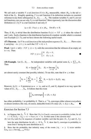
![324 7.3 Convergence ofrandom variables
3. Let {Sn : n 2: O} be a simple random walk which moves to the right with probability p at each
step, and suppose that So = O. Write Xn = Sn - Sn-I .
(a) Show that {Sn = 0 i.o. } is not a tail event of the sequence {Xn }.
(b) Show that lP'(Sn = 0 i.o.) = 0 if p # i.
(c) Let Tn = Sn/.,;n, and show that
{lim inf Tn ':::: -x} n {lim sup Tn 2: x}
n----+oo n----+oo
is a tail event of the sequence {Xn }, for all x >0, and deduce directly that lP'(Sn = 0 i.o.) = I if
_ I
p - 2 ·
4. Hewitt-Savage zero-one law. Let Xl.X2,. . . be independent identically distributed random
variables. The event A, defined in terms of the Xn, is called exchangeable if A is invariant un
der finite permutations of the coordinates, which is to say that its indicator function fA satisfies
fA(XI,X2,...,Xn,. . . ) = fA(Xil,Xi2,...,Xin,Xn+I,. . . ) for all n 2: 1 and all permutations
(ii , i2, . . . , in) of ( 1 , 2, . . . , n). Show that all exchangeable events A are such that either lP'(A) = 0
or lP'(A) = 1 .
5. Returning to the simple random walk S ofExercise (3), show that {Sn = 0 i.o.} i s an exchangeable
event with respect to the steps of the walk, and deduce from the Hewitt-Savage zero-one law that it
has probability either 0 or 1 .
6. Weierstrass's approximation theorem. Let f : [0, 1] --+ lR be a continuous function, and let
Sn be a random variable having the binomial distribution with parameters n and x. Using the formula
E(Z)= E(ZfA)+ E(ZfAc)with Z= f(x) - f(n-1 Sn) and A = {In-1 Sn - xl >8}, show that
lim sup !f(X) - t f(k/n) (
n
) xk(l _ x)n-k ! = O.
n---?oo o< <1 k
_X _ k=O
You have proved Weierstrass's approximation theorem, which states that every continuous function
on [0, 1] may be approximated by a polynomial uniformly over the interval.
7. Complete convergence. A sequence XI , X2,. . . of random variables is said to be completely
convergent to Xif
LlP'(IXn -XI > E) < 00 for all E >O.
n
Show that, for sequences of independent variables, complete convergence is equivalent to a.s. conver
gence. Find a sequence of (dependent) random variables which converges a.s. but not completely.
8. Let XI , X2 , . . . be independent identically distributed random variables with common mean JL
and finite variance. Show that
as n --+ 00.
9. Let {Xn : n 2: I } be independent and exponentially distributed with parameter 1 . Show that
(. Xn )
lP' hm sup -- = 1 = 1 .
n---?oo log n
10. Let {Xn : n 2: I } be independent N(O, 1) random variables. Show that:
(a) lP' (lim sup � = ../2) = 1 ,
n---?oo v log n](https://image.slidesharecdn.com/grimmettstirzaker-probabilityandrandomprocessesthirded2001-220507085451-bb31ac14/85/Grimmett-Stirzaker-Probability-and-Random-Processes-Third-Ed-2001-pdf-335-320.jpg)
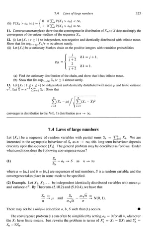
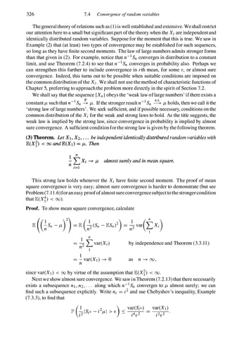
![328 7.4 Convergence ofrandom variables
(7) Theorem. Theindependentidenticallydistributedsequence {Xn}, withcommondistri
butionfunctionF, satisfies
1
n
- L Xi � I'-
n i=1
forsomeconstant1'-, ifandonlyifoneofthefollowingconditions(8) or(9) holds:
(8) nlP'(IXl l > n) -+ 0 and ( x dF -+ I'- asn -+ 00,
J[-n,n]
(9) thecharacteristicfunction<p(t)oftheXj isdifferentiableatt = 0 and<p'(0) = i1'-.
Ofcourse, the integral in (8) can be rewritten as
( xdF= E(XI J IXI I :'S n)lP'(IXl l :'S n) = E(XIIIIX1Isn}).
J[-n,n]
Thus, a sequence satisfies the weak law but not the strong law whenever (8) holds without
(6); as an example of this, suppose the Xj are symmetric (in that X1 and -X1have the same
distribution) but their common distribution function F satisfies
1
1 - F(x) '" -- as x -+ 00.
x logx
Some distributions fail even to satisfy (8).
(10) Example. Let the Xj have the Cauchy distribution with density function
1
f(x) =
n(l + x2)
.
Then the first part of (8) is violated. Indeed, the characteristic function of Un = n-1Sn is
and so Un itself has the Cauchy distribution for all values of n. In particular, (1) holds with
bn = n,an = 0, where S is Cauchy, and the convergence is in distribution. •
Exercises for Section 7.4
1. Let X2, X3, . . . be independent random variables such that
I
JP'(Xn = n) = JP'(Xn = -n) = -- ,
2n log n
1
JP'(Xn = 0) = 1 - --.
n log n
Show that this sequence obeys the weak law but not the strong law, in the sense that n-1'Ll Xi
converges to 0 in probability but not almost surely.
2. Construct a sequence {Xr : r :::: I } of independent random variables with zero mean such that
n-1 'L�=l Xr -+ -00 almost surely, as n -+ 00.
3. Let N be a spatial Poisson process with constant intensity A in ]Rd, where d :::: 2. Let S be the
ball of radius r centred at zero. Show that N(S) / I S I -+ A almost surely as r -+ 00, where l S I is the
volume of the ball.](https://image.slidesharecdn.com/grimmettstirzaker-probabilityandrandomprocessesthirded2001-220507085451-bb31ac14/85/Grimmett-Stirzaker-Probability-and-Random-Processes-Third-Ed-2001-pdf-339-320.jpg)
![7.5 The strong law 329
7.5 The strong law
This section is devoted to the proofof the strong law of large numbers.
(1) Theorem. Strong law of large numbers. Let Xl, X2, . . . be independent identically
distributed random variables. Then
1 n
- LXi -* JL almost surely, as n -* 00,
n j==l
forsome constantJL, ifand only ifEIXI I < 00. In this case JL = EX1.
The traditional proofofthis theorem is long and difficult, andproceeds by a generalization
of Chebyshov's inequality. We avoid that here, and give a relatively elementary proof which
is an adaptation ofthemethod used to prove Theorem (7.4.3). We make use ofthe technique
oftruncation, used earlier in the proofof the large deviation theorem (5.1 1.4).
Proof. Suppose first that the Xi are non-negative random variables with EIXII = E(XI) <
00, and write J,L = E(X]). We 'truncate' the Xnto obtain a new sequence {Yn}given by
(2)
Note that
n n
by the result of Problem (4.14.3). Of course, lP'(Xn :::: n) = lP'(XI :::: n) since the Xi are
identically distributed. By the first Bore1--Cantelli lemma (7.3.10a),
and so
(3)
lP'(Xn =1= Ynfor infinitely many values of n) = 0,
1
n a.s.
-L(Xi -Yj) � 0 as n -+ 00;
n i=1
thus it will suffice to show that
(4)
1
n
" y a.s.
-
� i � J,L
n i=]
as n -+ 00.
We shall need the following elementary observation. Ifa > 1 and th = LakJ , the integerpart
ofak, then there exists A > 0 such that
(5)
00 1 A
"
- < - for m :::: 1 .
� R2 - R2
k=m Pk Pm](https://image.slidesharecdn.com/grimmettstirzaker-probabilityandrandomprocessesthirded2001-220507085451-bb31ac14/85/Grimmett-Stirzaker-Probability-and-Random-Processes-Third-Ed-2001-pdf-340-320.jpg)
![330 7.5 Convergence ofrandom variables
This holds because, for large m, the convergent series on the left side is 'nearly' geometric
with first term f3;;/. Note also that
(6)
f3k+l
-- -+ a as k-+ 00.
f3k
Write S� = L:7=1 Yi. For a > 1 , E > 0, use Chebyshov's inequality to find that
(7) � ( 1 , , ) 1 � 1 ,
L..., lP' -ISpn -lE(Sp)1 > E ::::
E2 L..., 2 var(Sp)
n=l f3n n=l f3n
I 00 1 Pn
= 2" L 2 Lvar(Yi) by independence
E n=l f3n i=l
A 00 1
< -'" -lE(Y.2)
- E2 L..., j2 !
i=l
by changing the order of summation and using (5).
Let Bij = {j - 1 :::: Xi < j}, and note that lP'(Bij) = lP'(Blj). Now
(8)
Combine (7) and (8) and use Theorem (7.2.4c) to deduce that
(9)
Also,
1 [ , ' ] a.s.
f3n Spn -lE(Sp) ----+ 0 as n -+ 00.
lE(Yn) = lE(XnI{Xn<n}) = lE(XII{xl<n}) -+ lE(Xl) = JL
as n -+ 00, by monotone convergence (5.6.12). Thus
(remember the hint in the proofof Corollary (6.4.22)), yielding from (9) that
(10)
] S' a.s.
- " ----+ JL as n -+ 00;
f3n pn](https://image.slidesharecdn.com/grimmettstirzaker-probabilityandrandomprocessesthirded2001-220507085451-bb31ac14/85/Grimmett-Stirzaker-Probability-and-Random-Processes-Third-Ed-2001-pdf-341-320.jpg)
![7.5 The strong law 331
this is a partial demonstration of (4). In order to fill in the gaps, use the fact that the Yi are
non-negative, implying that the sequence {S�}is monotonic non-decreasing, to deduce that
1 1 1
(11) --SfJ' < -S' < -SfJ' if f3n :::: m :::: f3n+l .
f3n+I n - m m - f3n n+1
Let m -+ 00 in (1 1) and remember (6) to find that
(12)
1 1
a-I
/J. :::: lim inf -S� :::: lim sup -S� :::: a/J. almost surely.
m---'>oo m m---'>oo m
This holds for all a > 1 ; let a -i- 1 to obtain (4), and deduce by (3) that
(13)
1
n
'""' a.s.
- L..- Xi ----+ /J. as n -+ 00
n i=1
whenever the Xi are non-negative. Now proceed exactly as in the proof of Theorem (7.4.3)
in order to lift the non-negativity condition. Note that we have proved the main part of the
theorem without using the full strength of the independence assumption; we have used only
the fact that the Xi are pairwise independent.
In order to provethe converse, suppose that n-I I:?=I Xi � /J.. Then n-IXn � 0by
the theory ofconvergentreal series, and the second Borel-Cantelli lemma (7.3.lOb) gives
LlP'(IXnl 2: n) < 00,
n
since the divergence of this sum would imply that lP'(n-I IXnI 2: 1 i.o.) = 1 (only here do we
use the full assumption of independence). By Problem (4.14.3),
00 00
n=1 n=1
and hence lEIXI I < 00, which completes the proofofthe theorem. •
Exercises for Section 7.5
1. Entropy. The interval [0, I ] is partitioned into n disjoint sub-intervals with lengths PI , P2, . . . ,
Pn, and the entropy of this partition is defined to be
n
h = - L Pi log Pi ·
i=1
Let XI , X2, . . . be independent random variables having the unifonn distribution on [0, I ], and let
Zm (i) be the number of the XI , X2, . . . , Xm which lie in the ith interval of the partition above. Show
that
n
R - IT
Zm(i)
m - Pi
i=1
satisfies m-I log Rm -+ -h almost surely as m -+ 00.
2. Recurrentevents. Catastrophes occur at the times TI , T2, . . . where Ti =XI + X2+ . . . +Xi and
the Xi are independent identically distributed positive random variables. Let N(t) =max {n : Tn :::: t}
be the number of catastrophes which have occurred by time t. Prove that if E(XI ) < 00 then
N(t) -+ 00 and N(t)/t -+ I /E(XI ) as t -+ 00, almost surely.
3. Random walk. Let XI , X2, . . . be independent identically distributed random variables taking
values in the integers Z and having a finite mean. Show that the Markov chain S = {Sn} given by
Sn =�'{ Xi is transient if E(XI ) =f. O.](https://image.slidesharecdn.com/grimmettstirzaker-probabilityandrandomprocessesthirded2001-220507085451-bb31ac14/85/Grimmett-Stirzaker-Probability-and-Random-Processes-Third-Ed-2001-pdf-342-320.jpg)
![336 7.7 Convergence ofrandom variables
(9) Example. Let XI , X2, . . . be independent variables with zero means, finite variances,
and partial sums Sn = L:7=1 Xi. Define
Then
E(Tn+1 I XI, . . . , Xn) = E(S; + 2SnXn+l + X;+l IXI, . . . , Xn}
= Tn + 2E(Xn+I)E(Sn I Xl, . . . , Xn) + E(X;+I)
by independence
Thus {Tn} is not a martingale, since it only satisfies (4)with :::: in place of =; it is called a
'submartingale', and has properties similar to those of a martingale. •
Theseexamples show thatmartingales areall around us. They areextremely usefulbecause,
subject to a condition on their moments, they always converge; this is 'Doob's convergence
theorem' and is the main result of the next section. Martingales are explored in considerable
detail in Chapter 12.
Finally, here are some properties of conditional expectation. You neednotread them now,
butmayreferback to themwhen necessary. Recall thatthe conditional expectation ofX given
Y is defined by
E(X I Y) = 1jI(Y) where ljI(y) = E(X I Y = y)
is the mean of the conditional distribution of X given that Y = y. Most of the conditional
expectations in this chapter take the form E(X I V),the mean value of X conditional on the
values of the variables in the random vector Y = (Yl, Y2, . . . , Yn). We stress that E(X I Y)
is a function ofY alone. Expressions such as 'E(X I Y) = Z' should sometimes be qualified
by 'almost surely' ; we generally omit this qualification.
(10) Lemma.
(a) E(XI + X2 I Y) = E(XI I Y) + E(X2 I V).
(b) E(Xg(Y) I Y) = g (Y)E(X I Y) for (measurable)functions g : Rn -+ JR.
(c) E(X I h(Y)) = E(X I Y) ifh : Rn -+ JRn is one-one.
Sketch proof.
(a) This depends on the linearity of expectation only.
(b) E(Xg (Y) I Y = y) = g (y)E(X I Y = y).
(c) Roughly speaking, knowledge ofY is interchangeable with knowledge ofh(Y), in that
Y(w) = y if and only if h(Y(w)) = h(y), for any W E Q. •
(11) Lemma. Tower property. E[E(X I Yl, Y2) IYI] = E(X IYI).
Proof. Just write down these expectations as integrals involving conditional distributions to
see that the result holds. It is a more general version of Problem (4.14.29). •](https://image.slidesharecdn.com/grimmettstirzaker-probabilityandrandomprocessesthirded2001-220507085451-bb31ac14/85/Grimmett-Stirzaker-Probability-and-Random-Processes-Third-Ed-2001-pdf-347-320.jpg)
![7.7 Martingales 337
Sometimes we considerthe mean value E(X I A)ofa random variable X conditional upon
the occurrence of some event Ahaving strictly positive probability. This is just the mean of
the corresponding distribution function FXIA(x) = lJD(X :s x I A). We can think ofE(X I A)
as a constant random variable with domain A � Q; it is undefined at points W E AC• The
following result is an application ofLemma (1.4.4).
(12) Lemma. If{Ri : 1 :s i :s n} is apartition ofAthen
n
E(X I A)lP(A) = LE(X I Bi)lP(Ri).
i=l
You may like the following proof:
E(XIA) = E(X L IB.) = LE(XIB.).
I I
Sometimes we consider mixtures of these two types ofconditional expectation. These are
of the form E(X I Y, A) where X, Yl, . . . , Yn are random variables and A is an event. Such
quantities are defined in the obvious way and have the usual properties. For example, (11)
becomes
(13) E(X I A) = E[E(X I Y, A)I AJ.
We shall make some use ofthe following fact soon. If, in (13), Ais an event which is defined
in terms ofthe Yi (such as A = {Yl :s I} or A = {IY2Y3 - Y41 > 2}) then it is not difficult to
see that
(14) E[E(X I Y) I A] = E[E(X I Y, A) I A];
just note that evaluating the random variable E(X I Y, A)at a point W E Q yields
E(X I Y, A)(w){ � E(X I Y)(w) if w E A
IS undefined if w¢. A.
The sequences {Sn} ofthis section satisfy
(15)
(16) Lemma. If{Sn} satisfies (15)then:
(a) E(Sm+n I Xl , . . . , Xm) = Sm for all m, n :::: 1,
(b) E(Sn) = E(Sl)for all n.
Proof.
(a) Use (11)with X = Sm+n, YI = (XI, . . . , Xm), and Y2 = (Xm+l, . . . , Xm+n-d to
obtain
E(Sm+n I Xl, . . . , Xm) = E[E(Sm+n I Xl, . . . , Xm+n-d I Xl, . . . , Xm]
= E(Sm+n-l I Xl, . . . , Xm)
and iterate to obtain the result.
(b) E(Sn) = E(E(Sn I Xl)) = E(S]) by (a). •
For a more satisfactory account of conditional expectation, see Section 7.9.](https://image.slidesharecdn.com/grimmettstirzaker-probabilityandrandomprocessesthirded2001-220507085451-bb31ac14/85/Grimmett-Stirzaker-Probability-and-Random-Processes-Third-Ed-2001-pdf-348-320.jpg)
![7.8 Martingale convergence theorem 339
Proofof(2). Let Ao = Q, Ak = {lSi I < E for all i :-::: k}, and let Bk = Ak-l n {ISkl :::: E} be
the eventthat lSi I :::: E forthe first time when i = k. Then
Therefore
(3)
However,
n n
lE(S;) = LlE(S;IB.) + lE(S;IAn) :::: LlE(S;IB,).
i=1 i=1
lE(S;IB,) = lE( Sn - Si + Sd2IB,)
= lE( Sn - Si)2IB,) + 2lE( Sn - SdS;lB,) + lE(S;IB.)
= a + fJ + y, say.
Note that a :::: 0 and y :::: E2lP'(Bi), because lSi I :::: E if Bi occurs. To deal with fJ, note that
lE((Sn - Si)S;lB,) = lE[S;lB,lE(Sn - Si I X1 , · · · , Xd] by Lemma (7.7. lOb)
= 0 by Lemma (7.7.16a),
since Bi concerns XI, . . . , Xi only, by the discussion after (7.7.4). Thus (3) becomes
and theresult is shown. •
Proofof (1). First note that Sm and (Sm+n - Sm) are uncorrelated whenever m, n :::: 1, since
by Lemma (7.7.16). Thus
(4)
It follows that {lE(S;)} is a non-decreasing sequence, whichis bounded above, bythe assump
tion in (1); hence we may suppose thatthe constant Mis chosen such that
We shall show that the sequence {Sn(w) : n :::: I} is almost-surely Cauchy convergent
(see the notes on Cauchy convergence after Example (7.2.2)). Let C = {w E Q : {Sn(w)}](https://image.slidesharecdn.com/grimmettstirzaker-probabilityandrandomprocessesthirded2001-220507085451-bb31ac14/85/Grimmett-Stirzaker-Probability-and-Random-Processes-Third-Ed-2001-pdf-350-320.jpg)
![340 7.8 Convergence ofrandom variables
is Cauchy convergent}. For W E C, the sequence Sn(w) converges as n --+ 00 to some limit
S(w), and we shall show that lP'(C) = 1. Note that
C = {YE > 0, 3m such that ISm+i - Sm+j l < E for all i, j ::::: I }.
By the triangle inequality
so that
C = {YE > 0, 3m such that ISm+i - Sml < E for all i ::::: I }
= n U{ISm+i - Sml < E for all i ::::: 1}.
E>O m
The complement of Cmay be expressed as
E>O m E>O m
where Am(E) = {ISm+i - Sml ::::: E for some i ::::: I}. Now Am(E) S; Am(E/) if E ::::: E/, so that
In order to prove that lP'(CC) = 0 as required, it suffices to show that lP'(Am(E» --+ 0 as
m --+ 00 for all E > O. To this end we shall use the Doob-Kolmogorov inequality.
For a given choice of m, define the sequence Y = {Yn : n ::::: I} by Yn = Sm+n - Sm. It
may be checked that Y is a martingale with respect to itself:
lE(Yn+l I Yl, . . . , Yn) = lE[lE(Yn+l I Xl, . . . , Xm+n) I Yl, . . . , Yn]
= lE(Yn I Yl, . . . , Yn) = Yn
by Lemma (7.7.1 1) and the martingale property. We apply the Doob-Kolmogorov inequality
(2) to this martingale to find that
Letting n --+ 00 and using (4)we obtain
and hence lP'(Am(E» --+ 0as m --+ 00 as required for almost-sure convergence. We have
proved that there exists a random variable S such that Sn � S.](https://image.slidesharecdn.com/grimmettstirzaker-probabilityandrandomprocessesthirded2001-220507085451-bb31ac14/85/Grimmett-Stirzaker-Probability-and-Random-Processes-Third-Ed-2001-pdf-351-320.jpg)
![344 7.9 Convergence ofrandom variables
such a Y? The answer is yes, and furthermore there is (essentially) a unique such Y in H. In
proving this we shall make use of two properties of H,that it is a linear space, and that it is
closed (with respect to the norm II.112);that is to say, for Z1,Z2,. . . E Hand aI,a2,... ER
(7) a1Z1+ a2Z2+ . . . + anZn E H, and
(8) if IIZm -Zn112 -+ 0as m,n -+ 00,there exists Z E Hsuch that Zn � Z.
(See Exercise (7.9.6a).) More generally, we call a set Hofrandom variables a closedlinear
space(with respect to II . 112)if IIX112 < 00for all X E H,and Hsatisfies (7) and (8).
(9) Theorem. LetHbeaclosedlinearspace(withrespectto11·112)ofrandomvariables. Let
Ybearandomvariableon(Q, :F, JP')withfinitevariance. ThereexistsarandomvariableY
inHsuchthat
(10) IIY-YII2 ::s IIY-ZII2 forallZ E H,
andwhichisuniqueinthesensethatJP'(Y= Y) = lforanyl'E HwithllY-l'lI2 = IIY-YII2.
Proof. Let d = inf{IIY - ZII2 : Z E H}, and find a sequence Zl,Z2,. . . in H such that
limn--+oo IIY-Znll2 = d. Now, for any A, B E H,the 'parallelogram rule' holdst:
to show this, just expand the right side. Note that !(A + B) E Hsince His a linear space.
Setting A = Zn,B = Zm,we obtain using the definition of dthat
IIZm -Znll� ::S 2(IIY-Zmll�-2d+ IIY-Znll�) -+ 0 as m,n -+ 00.
Therefore IIZm -Znll2 -+ 0, so that there exists YE H such that Zn � Y;it is here that
we use the fact (8) that His closed. It follows by the triangle inequality (4)that
so that Ysatisfies (10).
Finally, suppose that l' E Hsatisfies IIY-l'II2 = d. Apply (11)with A = l', B = Y, to
obtain
Ill'-YII� = 4[d2- IiY - !(l'+ Y)Ii�] ::s 4(d2-d2) = O.
Hence E«l'-y)2) = 0and so JP'(Y= l')= 1. •
(12) Example. Let Y have mean /1 and variance a2. With no information about Y, it is
appropriate to ask for the real number h which minimizes IIY -h1l2. Now IIY - hll� =
E«Y -h)2) = a2+ (/1 -h)2, so that /1 is the best predictor of Y. The set Hof possible
estimators is the real line lR. •](https://image.slidesharecdn.com/grimmettstirzaker-probabilityandrandomprocessesthirded2001-220507085451-bb31ac14/85/Grimmett-Stirzaker-Probability-and-Random-Processes-Third-Ed-2001-pdf-355-320.jpg)
![7.9 Prediction and conditional expectation 345
(13) Example. Let Xl , X2, . . . be uncorrelated random variables with zero means and unit
variances. It is desired to findthe bestpredictorof Y amongstthe class oflinear combinations
of the Xi.Clearly
E ((Y -�aiXir) = E(y2) -2 �aiE(Xi Y) + �al
I I I
= E(y2) + �]ai- E(Xiy)]2 - LE(Xi y)2.
i i
This is a minimum when ai= E(Xi Y) for all i,so that f = Li XiE(Xi Y). (Exercise: Prove
that E(YZ) < 00.) This is seen best in the following light. Thinking of the Xi as orthogonal
(that is, uncorrelated) unit vectors in the space H of linear combinations of the Xi, we have
found that f is the weighted average of the Xi, weighted in proportion to the magnitudes of
their 'projections' onto Y . The geometry of this example is relevant to Theorem (14). •
(14) Projection theorem. LetH beaclosedlinearspace(withrespectto II . 112) ofrandom
variables, andlet Y satisfyE(y2) < 00. LetM E H. Thefollowingtwostatementsare
equivalent:
(15)
(16)
E( Y - M)Z) = 0 forallZ E H,
II Y - MII2 ::s II Y - ZII2 forallZ E H.
Here is the geometrical intuition. Let L2(Q , F, JP') be the set of random variables on
(Q, F, JP') having finite second moment. Now H is a linear subspace of L2(Q, F, JP'); think
of H as a hyperplane in a vector space of very large dimension. If Y � H then the shortest
route from Y to H is along the perpendicular from Y onto H. Writing f for the foot of
this perpendicular, we have that Y -f is perpendicular to any vector in the hyperplane H.
Translatin1 this geometrical remark back into the language ofrandom variables, we conclude
that (Y - Y, Z) = o forall Z E H, where (U, V) is thescalarproduct in L2(Q, F, JP') defined
by (U,V) = E(UV). These remarks do not of course constitute a proofof the theorem.
Proof. Suppose first that M E H satisfies (15). Then, for M' E H,
E( Y - M')2) = E( Y - M + M - M?)
= E( Y - M)2) + E( M - M?)
by (15), since M -M' E H; therefore II Y - MII2 ::s II Y - M'1I2 for all M' E H.
Conversely, suppose that M satisfies (16), but that there exists Z E H such that
E((Y - M)Z) = d > O.
Wemay assume withoutlossofgeneralitythatE(Z2) = 1 ; otherwisereplace Z by Z/JE(Z2),
noting that E(Z2) i= 0since JP'(Z = 0)i= 1. Writing M' = M + dZ, we have that
E( Y - M?) = E( Y - M + M - M')2)
= E((Y - M)2) - 2dE((Y - M)Z) + d2E(Z2)
= E( Y - M)2) - d2,
in contradiction ofthe minimality ofE« Y - M)2). •](https://image.slidesharecdn.com/grimmettstirzaker-probabilityandrandomprocessesthirded2001-220507085451-bb31ac14/85/Grimmett-Stirzaker-Probability-and-Random-Processes-Third-Ed-2001-pdf-356-320.jpg)
![346 7.9 Convergence ojrandom variables
It is only a tiny step from the projection theorem (14) to the observation, well known to
statisticians, that the best predictor of Y given X is just the conditional expectation E(Y I X).
This fact, easily proved directly (exercise),follows immediately from the projection theorem.
(17) Theorem. LetX andY berandomvariables, andsupposethatE(y2) < 00. Thebest
predictorofY givenX istheconditionalexpectationE(Y I X).
Proof. Let H be the closed linear space of functions of X having finite second moment.
Define 1/t(x) = E(Y I X = x). Certainly 1/t(X) belongs to H, since
where we have used the Cauchy-Schwarz inequality. On the other hand, for Z = h(X) E H,
E([Y - 1/t(X)]Z) = E(Yh(X» - E(E(Y I X)h(X»)
= E(Yh(X» - E(E(Yh(X) I X»)
= E(Yh(X» - E(Yh(X») = 0,
using the elementary fact that E(Yh(X) I X) = h(X)E(Y I X). Applying the projection
theorem, we find that M = 1/t(X) (= E(Y I X» minimizes II Y - MII2 for M E H, which is
the claim of the theorem. •
Here is an important step. We may take the conclusion of (17) as a definition of the
conditional expectation E(Y I X): if E(y2) < 00,the conditionalexpectationE(Y I X) of Y
given X is defined to be the best predictor of Y given X.
There are two major advantages ofdefining conditional expectation in this way. First, itis
a definition which is valid for all pairs X, Y such that E(y2) < 00,regardless of their types
(discrete, continuous, and so on). Secondly, it provides a route to a much moregeneral notion
of conditional expectation which turns out to be particularlyrelevantto the martingaletheory
of Chapter 12.
(18) Example. Let X = {Xi : i E l} be a family of random variables, and let H be the
space of all functions of the Xi with finite second moments. If E(y2) < 00,the conditional
expectationE(Y I Xi, i E I) of Y given the Xi is defined to be the function M = 1/t(X) E H
which minimizes the mean squared error II Y - MII2 over all M in H. Note that 1/t(X) satisfies
(19) E([Y - 1/t(X)]Z) = 0 for all Z E H,
and 1/t(X) is unique in the sense that J.P'(1/t(X) = N) = 1 if II Y - 1/t(X) 1I2 = II Y - NII2 forany
N E H. We note here that, strictly speaking, conditional expectations are not actually unique;
this causes no difficulty, and we shall therefore continue to speak in terms of theconditional
expectation. •
We move on to an important generalization ofthe idea ofconditionalexpectation, involving
'conditioning on a a-field' . Let Y be a random variable on (Q, F, J.P') having finite second
moment, and let g. be a sub-a-field of F. Let H be the space of random variables which
are g.-measurable and have finite second moment. That is to say, H contains those random
variables Z such that E(Z2) < 00and {Z ::s z} E g. for all Z E R. It is not difficult to see that
H is a closed linear space with respect to II . 112. We have from (9) that there exists an element](https://image.slidesharecdn.com/grimmettstirzaker-probabilityandrandomprocessesthirded2001-220507085451-bb31ac14/85/Grimmett-Stirzaker-Probability-and-Random-Processes-Third-Ed-2001-pdf-357-320.jpg)
![7.9 Prediction and conditional expectation 347
M ofHsuchthat IIY-M112 .::::: IIY-Z112forallZ E H,andfurthermoreM isunique(inthe
usualway)withthisproperty. WecallM the 'conditionalexpectationofY giventhea-field
g,', writtenlE(Y I g,).
This is amore general definition ofconditionalexpectationthan thatobtainedby condi
tioningonafamilyofrandomvariables (as inthepreviousexample). To seethis, take g,to
bethesmallesta-fieldwithrespecttowhicheverymemberofthefamily X = {Xi : i E I}
ismeasurable. Itis clearthatlE(Y I g,) = lE(Y I Xi, i E /),inthe sensethattheyareequal
withprobability 1.
Wearriveatthefollowingdefinitionbyuseoftheprojectiontheorem(14).
(20) Definition. Let (Q, F, JP') be aprobability space, and let Y be arandomvariable sat
isfyinglE(y2) < 00. Ifg, is a sub-a-fieldofF, theconditional expectation lE(Y I g,) is a
g,-measurablerandomvariable satisfying
(21) lE([Y -lE(Y I g,)]Z) = 0 forall Z E H,
whereHisthecollectionofall g,-measurablerandomvariableswithfinite secondmoment.
TherearecertainmembersofHwithparticularlysimpleform,beingtheindicatorfunctions
ofeventsin g,. Itmaybeshownwithoutgreatdifficultythatcondition(21) maybereplaced
by
(22) lE([Y -lE(Y I g,)]IG) = 0 forall G E g,.
SettingG = Q, wededucetheimportantfactthat
(23) lE(lE(Y I g,») = lE(Y).
(24) Example. Doob's martingale. (Though some ascribethis toLevy.) Let Y havefinite
secondmoment,andletXI, X2, ... beasequenceofrandomvariables. Define
Yn = lE(Y I XI , X2, · · · , Xn).
Then {Yn} is a martingale with respect to {Xn}. To show this itis necessary to prove that
lElYnl < oo andlE(Yn+1 I XI, X2, ... , Xn) = Yn. CertainlylElYnl < oo, sincelE(Y;) < 00.
Fortheotherpart, let Hn bethe spaceoffunctionsofXI , X2, ... , Xn having finite second
moment. Wehaveby(19)that,forZ E Hn,
0 = lE((Y - Yn)Z) = lE((Y - Yn+1 + Yn+1 - Yn)Z)
= lE( Yn+1 - Yn)Z) since Z E Hn <;: Hn+l.
ThereforeYn = lE(Yn+1 I XI , X2, ... , Xn)·
Hereisamoregeneralformulation.LetYbearandomvariableon(Q, F, JP') withlE(y2) <
00,andlet {g,n : n :::: I} beasequenceofa-fieldscontainedin F andsatisfying g,n <;: g,n+1
foralln. Suchasequence {g,n} iscalledafiltration;inthecontextofthepreviousparagraph
wemighttake g,n tobethe smallest a-fieldwith respectto which XI, X2, ... , Xn areeach
measurable. Wedefine Yn = lE(Y I g,n). Asbefore {Yn} satisfies lElYnl < 00andlE(Yn+1 I
g,n) = Yn; suchasequenceiscalleda 'martingalewithrespecttothefiltration {g,n}'. •](https://image.slidesharecdn.com/grimmettstirzaker-probabilityandrandomprocessesthirded2001-220507085451-bb31ac14/85/Grimmett-Stirzaker-Probability-and-Random-Processes-Third-Ed-2001-pdf-358-320.jpg)
![348 7.9 Convergence ofrandom variables
This newtype ofconditionalexpectationhasmany useful properties. We single outone
ofthese, namely thepull-throughproperty,thus named since it involves arandomvariable
beingpulledthroughaparanthesis.
(25)Theorem. LetY havefinitesecondmomentandletfj,beasub-a-fieldofthea-fieldF.
ThenJE(XY I fj,) = XJE(Y I fj,)forallfj,-measurablerandomvariablesX withfinitesecond
moments.
Proof. LetX be fj,-measurablewithfinitesecondmoment. Clearly
Z = JE(XY I fj,) - XJE(Y I fj,)
is fj,-measurableandsatisfies
Z = X[Y - JE(Y I fj,)] - [XY - JE(XY I fj,)]
sothat,forG E fj"
JE(ZIG) = JE([Y - JE(Y I fj,)]XIG) - JE([XY - JE(XY I fj,)]/G) = 0,
thefirsttermbeingzerobythefactthatXIG isfj,-measurablewithfinitesecondmoment,and
the secondbythedefinitionofJE(XY I fj,). Any fj,-measurablerandomvariable Z satisfying
JE(ZIG) = 0 forallG E fj,is suchthatlP'(Z = 0) = 1 GustsetGl = {Z > OJ,G2= {Z < O}
intum),andthe resultfollows. •
In all our calculations so far, we have used the norm II . 112, leading to a definition of
JE(Y I fj,) forrandomvariablesY withJE(y2) < 00. Thisconditionoffinitesecondmomentis
ofcoursetoo strongingeneral,andneedstobereplacedbythenaturalweakerconditionthat
JEIYI < 00. One way ofdoingthis wouldbetoreworkthepreviousargumentsusinginstead
the norm II . 111. An easier route is to use the technique of 'truncation' as in the following
proof.
(26) Theorem. Let Y bea randomvariableon (Q , :F, lP') withJEIYI < 00, andletfj, bea
sub-a-fieldof:F. ThereexistsarandomvariableZ suchthat:
(a) Z isfj,-measurable,
(b) JEIZI < 00,
(c) JE« Y - Z)/G) = OforallG E fj,.
Zisuniqueinthesensethat,foranyZ'satisfying(a),(b),and(c),wehavethatlP'(Z= Z') = 1.
TherandomvariableZ inthetheoremiscalledthe 'conditionalexpectationofY givenfj,',
andiswrittenJE(Y I fj,). Itisanexercisetoprovethat
(27) JE(XY I fj,) = XJE(Y I fj,)
for all fj,-measurable X, whenever both sides exist, and also that this definition coincides
(almostsurely)withthepreviousonewhen Y hasfinitesecondmoment. Ameaningfulvalue
can be assignedto JE(Y I fj,) underthe weaker assumptionon Y thateitherJE(Y+) < 00or
JE(Y-) < 00.](https://image.slidesharecdn.com/grimmettstirzaker-probabilityandrandomprocessesthirded2001-220507085451-bb31ac14/85/Grimmett-Stirzaker-Probability-and-Random-Processes-Third-Ed-2001-pdf-359-320.jpg)
![7.9 Prediction and conditional expectation 349
Proof. Suppose first that Y ::::: 0 and IEIYI < 00. Let Yn = min{Y, n}, so that Yn t Y as
n -+ 00. Certainly lE(Y;) < 00,and hence we may use (20) to findthe conditional expectation
IE(Yn I g,), a g,-measurable random variable satisfying
(28) 1E([Yn - IE(Yn I g,)]IG) = 0 for all G E g,.
Now Yn < Yn+l, and so we may take IE(Yn I g,) :'S IE(Yn+l I g,) ; see Exercise (7.9.4iii).
Hence limn---+oo IE(Yn I g,) exists, and we write IE(Y I g,) for this limit, a g,-measurable random
variable. By monotone convergence (5.6. 12) and (23), IE(YnIG) tIE(YIG), and
1E[IE(Yn I g,)/G] tIE[IE(Y I g,)IG] = IE[IE(YIG I g,)] = IE(YIG),
so that, by (28), IE([Y - IE(Y I g,)]IG) = 0 for all G E g,.
Next we lift in the usual way the restriction that Y be non-negative. We express Y as
Y = y+ - Y- where y+ = max{Y, O} and Y- = - min{Y, O} are non-negative; we define
IE(Y I g,) = IE(Y+ I g,) - IE(Y- I g,). It is easy to check that IE(Y I g,) satisfies (a), (b), and
(c). To see the uniqueness, suppose that there exist two g,-measurable random variables ZI
and Z2 satisfying (c). Then IE((ZI - Z2)IG) = IE((Y - Y)IG) = 0 for all G E g,. Setting
G= {ZI > Z2} and G= {ZI < Z2} in tum, we find that JP'(Z1 = Z2) = 1 as required. •
Having defined IE(Y I g,), we can ofcourse define conditional probabilities also: if A E :F,
we define JP'(A I g,) = IE(lA I g,) . It may be checked that JP'(0 I g,) = 0, JP'(Q I g,) = 1 a.s.,
and JP'(U Ai I g,) = Li JP'(Ai I g,) a.s. for any sequence {Ai : i ::::: I} of disjoint events in :F.
It looks as though there should be a way of defining JP'(. I g,) so that it is a probability
measure on (Q , :F). This turns out to be impossible in general, but the details are beyond the
scope of this book.
Exercises for Section 7.9
1. Let Y be uniformly distributed on [- 1 , 1] and let X = y2.
(a) Find the best predictor of X given Y, and of Y given X.
(b) Find the best linear predictor of X given Y, and of Y given X.
2. Let the pair (X, Y) have a general bivariate normal distribution. Find JE(Y I X).
3. Let Xj , X2, . . . , Xn be random variables with zero means and covariance matrix V = (vij), and
let Y have finite second moment. Find the linear function h of the Xi which minimizes the mean
squared error JE{(Y - h(X1, " . ' Xn»2}.
4. Verify the following properties of conditional expectation. You may assume that the relevant
expectations exist.
(i) JE{JE(Y I fl.)) = JE(Y).
(ii) JE(aY + {3Z I fl.) = aJE(Y I fl.) + {3JE(Z I fl.) for a, {3 E JR.
(iii) JE(Y I fl.) :::: 0 if Y :::: O.
(iv) JE(Y I fl.) = JE{JE(Y I Jt) I fl.} if fI. � R.
(v) JE(Y I fl.) = JE(Y) if Y is independent of IG for every G E fl..
(vi) Jensen's inequality. g{JE(Y I fl.)} :'S JE{g(Y) I fl.} for all convex functions g.
(vii) If Yn � Y and I Yn I :'S Z a.s. where JE(Z) < 00, then JE(Yn I fl.) � JE(Y I fl.).
(Statements (ii)-(vi) are of course to be interpreted 'almost surely' .)
5. Let X and Y have joint mass function f(x, y) = {x(x + 1 ) )-1 for x = y = 1 , 2, . . " Show that
JE(Y I X) < 00 while JE(Y) = 00.](https://image.slidesharecdn.com/grimmettstirzaker-probabilityandrandomprocessesthirded2001-220507085451-bb31ac14/85/Grimmett-Stirzaker-Probability-and-Random-Processes-Third-Ed-2001-pdf-360-320.jpg)
![354 7. 1 1 Convergence ojrandom variables
for any integer f3 satisfying 1 ::s f3 < ex. This may be proved either directly or via Theorem
(3). First, if f3 is an integer satisfying 1 ::s f3 < ex , then {X� : n 2: I } is uniformly integrable
by (5), and furthermore X� � XfJ (easy exercise,or use Theorem (7.2. 18)). If it were the
case that X� � XfJ then Theorem (3) would imply the result. In any case, by the Skorokhod
representation theorem (7.2. 14), there exist random variables Y, Yl , Y2 , . . . having the same
distributions as X, XI , X2 , . . . such that Y! � yfJ. Thus IE(Y!) --+ IE(yfJ) by Theorem (3).
However, IE(Y!) = IE(X�) and IE(yfJ) = IE(XfJ), and the proof is complete. •
Exercises for Section 7 . 1 0
1. Show that the sum {Xn + Yn } of two uniformly integrable sequences {Xn} and {Yn} gives a
uniformly integrable sequence.
2. (a) Suppose that Xn � X where r 2: 1 . Show that {IXn lr : n 2: I } is uniformly integrable, and
deduce that E(X�) --+ E(Xr) if r is an integer.
(b) Conversely, suppose that {IXn lr : n 2: I } is uniformly integrable where r 2: 1 , and show that
Xn � X if Xn � X.
3. Let g : [0, (0) --+ [0, (0) be an increasing function satisfying g(x)/x --+ 00 as x --+ 00. Show
that the sequence {Xn : n 2: I } is uniformly integrable if sUPn E{g(IXn I)} < 00.
4. Let {Zn : n 2: O} be the generation sizes of a branching process with Zo = I , E(ZI ) = 1,
var(Zj ) =f. O. Show that {Zn : n 2: O} is not uniformly integrable.
p p p
5. Pratt's lemma. Suppose that Xn S Yn S Zn where Xn --+ X, Yn --+ Y, and Zn --+ Z. If
E(Xn) --+ E(X) and E(Zn) --+ E(Z), show that E(Yn) --+ E(Y).
6. Let {Xn : n 2: l } be a sequence of variables satisfying E(suPn IXn I) < 00. Show that {Xn} is
uniformly integrable.
1. Let Xn have density function
7.11 Problems
n 2: 1 .
With respect to which modes of convergence does Xn converge as n --+ oo?
2. (i) Suppose that Xn � X and Yn � Y, and show that Xn + Yn � X + Y. Show that the
corresponding result holds forconvergence in rth mean and in probability, but not in distribution.
(ii) Show that if Xn � X and Yn � Y then XnYn � XY. Does the corresponding result hold
for the other modes of convergence?
3. Let g : IR --+ IR be continuous. Show that g(Xn) � g(X) if Xn � X.
4. Let Yj , Y2 , . " be independent identically distributed variables, each of which can take any value
in {O, 1 , . . . , 9} with equal probability /0' Let Xn = 2:;=1 Yi 10-; . Show by the use ofcharacteristic
functions that Xn converges in distribution to theuniform distribution on [0, 1]. Deduce that Xn � Y
for some Y which is uniformly distributed on [0, 1].](https://image.slidesharecdn.com/grimmettstirzaker-probabilityandrandomprocessesthirded2001-220507085451-bb31ac14/85/Grimmett-Stirzaker-Probability-and-Random-Processes-Third-Ed-2001-pdf-365-320.jpg)
![7. 1 1 Problems
5. Let N(t) be a Poisson process with constant intensity on R
(a) Find the covariance of N(s) and N(t).
355
(b) Show that N is continuous in mean square, which is to say that E({N(t + h) - N(t)}2) -+ 0 as
h -+ o.
(c) Prove that N is continuous in probability, which is to say that lI"(IN(t + h) - N(t)1 > E) -+ 0 as
h -+ 0, for all E > O.
(d) Show that N is differentiable in probability but not in mean square.
6. Prove that n-I L:i=l Xi � 0 whenever the Xi are independent identically distributed variables
with zero means and such that E(Xi) < 00.
7. Show that Xn � X whenever L:n E(IXn - Xn < 00 for some r > O.
8. Show that if Xn � X then aXn + b � aX + b for any real a and b.
9. If X has zero mean and variance a2, show that
a2
lI"(X � t) �
-
2--
2 for t > O.
a + t
10. Show that Xn � 0 if and only if
11. The sequence {Xn } is said to be mean-square Cauchy convergent if E{(Xn - Xm)2} -+ 0 as
m, n -+ 00. Show that {Xn } converges in mean square to some limit X ifand only ifit is mean-square
Cauchy convergent. Does the corresponding result hold for the other modes of convergence?
12. Suppose that {Xn } is a sequence ofuncorrelatedvariables with zero means anduniformlybounded
. Sh th -I ",n X m.s. 0
vanances. ow at n L..i=l i � .
13. Let Xl , X2, . . . be independent identically distributed random variables with the common dis-
tribution function F, and suppose that F(x) < 1 for all x. Let Mn = max{XJ , X2, . . . , Xn } and
suppose that there exists a strictly increasing unbounded positive sequence ai , a2, . . . such that
11" (Mn/an � x) -+ H(x) for some distribution function H. Let us assume that H is continuous
with 0 < H(l) < 1 ; substantially weaker conditions suffice but introduce extra difficulties.
(a) Show that n[l - F(anx)] -+ - log H(x) as n -+ 00 and deduce that
1 - F(anx) log H(x)
-+ --=_C-.-
1 - F(an) log H(1)
ifx > O.
(b) Deduce that ifx > 0
1 - F(tx) log H(x)
-+ ---=--- as t -+ 00.
1 - F(t) log H(l)
(c) Set x = X,X2 and make the substitution
log H(eX)
g(x) =
log H(1)
to find that g(x + y) = g(x)g(y), and deduce that
H(x) =
{ �xp(-ax-.B) ifx � 0,
ifx < 0,](https://image.slidesharecdn.com/grimmettstirzaker-probabilityandrandomprocessesthirded2001-220507085451-bb31ac14/85/Grimmett-Stirzaker-Probability-and-Random-Processes-Third-Ed-2001-pdf-366-320.jpg)
![7.1 1 Problems 357
20. Let XI , X2, . . . be random variables satisfying var(Xn) < c for all n and some constant c. Show
that the sequence obeys the weak law, in the sense that n-1 Ll(Xi - lEXi) converges in probability
to 0, if the correlation coefficients satisfy either of the following:
(i) P(Xi, Xj) ::; 0 for all i =I- j,
(ii) P(Xi, Xj) -+ 0 as Ii - jl -+ 00.
21. Let XI , X2, . . . be independent random variables with common density function
f(x) = {O
c
x2 10g Ixl
if Ixl ::; 2,
if Ixl > 2,
where c is a constant. Show that the Xi have no mean, but n- 1 Ll=l Xi � 0 as n -+ 00. Show that
convergence does not take place almost surely.
22. Let Xn be the Euclidean distance between two points chosen independently and uniformly from
the n-dimensional unit cube. Show that lE(Xn)IIn -+ 1/.J6 as n -+ 00.
23. Let Xl, X2, . . . be independent random variables having the uniform distribution on [- 1, 1].
Show that
24. Let Xl, X2, . . . be independent random variables, each Xk having mass function given by
1
lP'(Xk =k) = lP'(Xk = -k) =
2k2 '
lP'(Xk = 1) =lP'(Xk = -1) = � (1 -
k
l
2 ) if k > 1.
Show that Un =Ll Xi satisfies UnlIn � N(O, 1) but var(UnlIn) -+ 2 as n -+ 00.
25. Let Xl, X2, ' " be random variables, and let N1, N2, ' " be random variables taking values in
the positive integers such that Nk � 00 as k -+ 00. Show that:
(i) if Xn � X and the Xn are independent of the Nk, then XNk � X as k -+ 00,
(ii) if Xn � X then XNk � X as k -+ 00.
26. Stirling's formula.
(a) Let a(k, n) =nkI(k - l) ! for 1 ::; k ::; n + 1. Use the fact that I -x ::; e-x ifx :::: O to show that
a(n - k, n)
::; e-k2/(2n)
a(n + l , n)
if k :::: O.
(b) Let X] , X2, . . . be independent Poisson variables with parameter 1, andlet Sn =Xl + . . . + Xn.
Define the function g : lR -+ lR by
{ -x
g(x) = 0
if O :::: x :::: -M,
otherwise,
where M is large and positive. Show that, for large n,
( {S n
}) e-n
lE g
n
;n = In
{a(n + l , n) - a(n - k, n) }](https://image.slidesharecdn.com/grimmettstirzaker-probabilityandrandomprocessesthirded2001-220507085451-bb31ac14/85/Grimmett-Stirzaker-Probability-and-Random-Processes-Third-Ed-2001-pdf-368-320.jpg)
![358
where k
formula:
7. 1 1 Convergence ofrandom variables
LMn 1/2J . Now use the central limit theorem and (a) above, to deduce Stirling's
n ! en
1 ---+ 1
nn+2 £
as n ---+ 00.
27. A bag contains red and green balls. A ball is drawn from the bag, its colour noted, and then it
is returned to the bag together with a new ball of the same colour. Initially the bag contained one
ball of each colour. If Rn denotes the number of red balls in the bag after n additions, show that
Sn = Rn/(n + 2) is a martingale. Deduce that the ratio of red to green balls converges almost surely
to some limit as n ---+ 00.
28. Anscombe's theorem. Let {Xi : i :::: I} be independent identically distributed random variables
with zero mean and finite positive variance 0-2, and let Sn = �'i Xi. Suppose that the integer-valued
random process M(t) satisfies t-I M(t) � () as t ---+ 00, where () is a positive constant. Show that
SM(t) � N(O, 1) and
o-$t
SM(t) � N(O, 1)
o-v'M(t)
You should not assume thatthe process M is independent ofthe Xi.
as t ---+ 00.
29. Kolmogorov's inequality. Let XI, X2, . . . be independent random variables with zero means,
and Sn = XI +X2 + . . . + Xn. Let Mn = maxI.sk.sn ISk l and show that E(S�IAk) > c2lP'(Ak) where
Ak = {Mk-I ::: c < Mk} and c > O. Deduce Kolmogorov's inequality:
c > O.
30. Let XI, X2, . . . be independent random variables with zero means, and let Sn = XI + X2 +
. . . + Xn. Using Kolmogorov's inequality or the martingale convergence theorem, show that:
(i) ��I Xi converges almost surely if ��I E(Xt) < 00,
(ii) if there exists an increasing real sequence (bn) such that bn ---+ 00, and satisfying the inequality
��I E(Xt)/bt < 00, then b;1 ��I Xk � 0 as n ---+ 00.
31. Estimating the transition matrix. The Markov chain Xo, X], . . . , Xn has initial distribution
fi = lP'(XO = i) and transition matrix P. The log-likelihood function ),,(P) is defined as ),,(P)
log(fxo PXO,Xt PX1 ,X2 ' " PXn-l ,Xn ). Show that:
(a) ),,(P) = log fxo + �i,j Nij log Pij where Nij is the number of transitions from i to j,
(b) viewed as a function ofthe Pij , ),,(P) is maximal when Pij = Pij where Pij = Nij /�k Nik,
(c) if X is irreducible and ergodic then Pij � Pij as n ---+ 00.
32. Ergodic theorem in discrete time. Let X be an irreducible discrete-time Markov chain, and let
JLi be the mean recurrence time of state i. Let Vi (n) = ��;::;J I[Xr=il be the number of visits to i up
to n - 1, and let f be any bounded function on S. Show that:
) -I V ( )
a.s. -1
(a n i n ---+ JLi as n ---+ 00,
(b) if JLi < 00 for all i, then
1 n-I
- L f(Xr) ---+ L f(i)/JLi as n ---+ 00.
n r=O iES
33. Ergodictheoremincontinuous time. LetXbeanirreduciblepersistentcontinuous-timeMarkov
chain with generator G and finite mean recurrence times JLj .
) Sh th
1
lot d a.s. 1
(a ow at - I[X(s)=j) s ---+ -- as t ---+ 00;
t 0 JLjgj](https://image.slidesharecdn.com/grimmettstirzaker-probabilityandrandomprocessesthirded2001-220507085451-bb31ac14/85/Grimmett-Stirzaker-Probability-and-Random-Processes-Third-Ed-2001-pdf-369-320.jpg)
![7. 1 1 Problems
(b) deduce that the stationary distribution Jl' satisfies trj = l/(fl-jgj);
(c) show that, if f is a bounded function o n S,
1 lot
- f(X(s» ds � L, 7rif(i)
t o .I
as t ---+ 00.
359
34. Tail equivalence. Suppose that the sequences {Xn : n 2: I} and {Yn : n 2: I} are tail equivalent,
which is to say that L:�] JP'(Xn I=- Yn) < 00. Show that:
(a) L:�] Xn and L:�] Yn converge or diverge together,
(b) L:�l (Xn - Yn) converges almost surely,
(c) ifthere exist a random variable X and a sequence an such that an t 00 and a;;1 L:�=1 Xr � X,
then
1 n
- L, Yr � X.
an r=]
35. Three series theorem. Let {Xn : n 2: l} be independent random variables. Show that L:�] Xn
converges a.s. if, for some a > 0, the following three series all converge:
(a) L:n JP'(lXn I > a),
(b) L:n var(XnIIIXnlsal),
(c) L:n E(XnIIIXnlsal)·
[The converse holds also, but is harder to prove.]
36. Let {Xn : n 2: I} be independent random variables with continuous common distribution function
F. We call Xk a record value for the sequence if Xk > Xr for 1 ::; r < k, and we write h for the
indicator function of the event that Xk is a record value.
(a) Show that the random variables h are independent.
(b) Show that Rm = L:k=l Ir satisfies Rm/log m � 1 as m ---+ 00.
37. Random harmonic series. Let {Xn : n 2: I} be a sequence of independent random variables
with JP'(Xn = 1) = JP'(Xn = - 1 ) = i. Does the series L:�=l Xr/r converge a.s. as n ---+ oo?](https://image.slidesharecdn.com/grimmettstirzaker-probabilityandrandomprocessesthirded2001-220507085451-bb31ac14/85/Grimmett-Stirzaker-Probability-and-Random-Processes-Third-Ed-2001-pdf-370-320.jpg)
![8
Random processes
Summary. This brief introduction to random processes includes elementary
previews of stationary processes, renewal processes, queueing processes, and
the Wiener process (Brownian motion). It ends with a discussion of the Kol
mogorov consistency conditions.
8.1 Introduction
Recall that a 'random process' X is a family {Xt : t E T} of random variables which
map the sample space Q into some set S. There are many possible choices for the index
set T and the state space S, and the characteristics of the process depend strongly upon
these choices. For example, in Chapter 6 we studied discrete-time (T = {O, 1 , 2, . . . }) and
continuous-time (T = [0, 00» Markov chains which take values in some countable set S.
Other possible choices for T include lRn and 7/.,
n, whilst S might be an uncountable set such
as lR. The mathematical analysis of a random process varies greatly depending on whether
S and T are countable or uncountable, just as discrete random variables are distinguishable
from continuous variables. The main differences are indicated by those cases in which
(a) T = {O, 1 , 2, . . . } or T = [0, 00),
(b) S = 7/., or S = lR.
There are two levels at which we can observe the evolution of a random process X.
(a) Each Xt is a function which maps Q into S. For any fixed W E Q, there is acorresponding
collection {Xt (w) : t E T} of members of S; this is called the realizationor sample
pathof X at w. We can study properties of sample paths.
(b) The Xt are not independent in general. If S � lR and t = (t1,t2,. . . , tn) is a vector
of members of T, then the vector (Xtl ' Xt2 ' . . . , Xtn) has joint distribution function
Ft : lRn � [0, 1] given by Ft(x) = lP'(Xtl .:::: Xl, . . . , Xtn .:::: Xn). The collection
{Ftl, as t ranges over all vectors of members of T of any finite length, is called the
collection offinite-dimensionaldistributions(abbreviated tofdds)of X, and it contains
all the information which is available about X from the distributions of its component
variables Xt . We can study the distributional properties of X by using its fdds.
These two approaches do not generally yield the same information about the process in
question, since knowledge ofthe fdds does not yield complete information aboutthe properties
of the sample paths. We shall see an example of this in the final section of this chapter.](https://image.slidesharecdn.com/grimmettstirzaker-probabilityandrandomprocessesthirded2001-220507085451-bb31ac14/85/Grimmett-Stirzaker-Probability-and-Random-Processes-Third-Ed-2001-pdf-371-320.jpg)
![362 8.2 Randomprocesses
Definitions similar to ( 1 ) and (2) hold for processes with T = R and for discrete-time
processes X = {Xn : n ::: OJ ; the autocovariance function of a weakly stationary discrete
time process Xis just a sequence {c(O, m) : m ::: O} of real numbers.
Weak stationarity interests us more than strong stationarity for two reasons. First, the
condition of strong stationarity is often too restrictive for certain applications; secondly, many
substantial and useful properties of stationary processes are derivable from weak stationarity
alone. Thus, the assertion that Xis stationaryshould be interpreted to mean that X is weakly
stationary. Of course, there exist processes which are stationary but not strongly stationary
(see Example (5» , and conversely processes without finite second moments may be strongly
stationary but not weakly stationary.
(4) Example. Markov chains. Let X = {X(t) : t ::: O} be an irreducible Markov chain
taking values in some countable subset Sof R and with a unique stationary distribution 7r .
Then (see Theorem (6.9.21»
IP'(X(t) = j IX (O) = i) -+ lrj as t -+ 00
for all i,j E S. The fdds of Xdepend on the initial distribution JL(O) of X (O), and it is not
generally true that Xis stationary. Suppose, however, that JL
(0) = 7r . Then the distribution
JL(t) of X(t) satisfies JL(t) = 7rPt = 7r from equation (6.9. 1 9), where {Pd is the transition
semigroup of the chain. Thus X(t)has distribution 7r for all t. Furthermore, if 0 < s < s+ t
and h > 0, the pairs (X(s),Xes + t» and (X(s + h),Xes + t + h» have the same joint
distribution since:
(a) X(s)and X(s+ h)are identically distributed,
(b) the distribution of X(s+ h)(respectively X(s+ t+ h» depends only on the distribution
of X(s) (respectively X(s+ t» and on the transition matrix Ph .
A similar argumentholds for collections ofthe X(u) which contain more than two elements,
and we have shown that Xis strongly stationary. •
(5) Example. Let A and B be uncorrelated (but not necessarily independent) random vari
ables, each of which has mean 0 and variance 1 . Fix a number ).. E [0, lr]and define
(6) Xn = A cos()..n) + Bsin()..n).
Then lEXn = 0 for all nand X = {Xn}has autocovariance function
c(m, m + n) = lE(XmXm+n)
= lE([A cos()..m) + Bsin()..m)][A cos{)..(m + n)}+ Bsin{)..(m + n)}J)
= lE(A2cos()..m) cos{)..(m + n)}+ B2sin()..m) sin{)..(m + n)})
= cos()..n)
since lE(AB) = O. Thus c(m, m + n) depends on nalone and so Xis stationary. In general
Xis not strongly stationary unless extra conditions are imposed on the joint distribution of A
and B;to see this for the case ).. = 1lr,simply calculate that
{XO, Xl , X2,X3,. . . } = {A , B,-A , -B,...}](https://image.slidesharecdn.com/grimmettstirzaker-probabilityandrandomprocessesthirded2001-220507085451-bb31ac14/85/Grimmett-Stirzaker-Probability-and-Random-Processes-Third-Ed-2001-pdf-373-320.jpg)
![8.2 Stationaryprocesses 363
which is strongly stationary ifand only ifthe pairs (A , B), (B, -A), and (-A , -B) have the
same joint distributions. It can be shown that X is strongly stationary for any A.if A and B
are N(O, 1) variables. The reason for this lies in Example (4.5.9), where we saw that normal
variables are independent whenever they are uncorrelated. •
Two major results in the theory of stationary processes are the 'spectral theorem' and the
'ergodic theorem' ; we close this section with a short discussion of these. First, recall from
the theory of Fourier analysis that any function f : R -+ R which
(a) is periodic with period 2][ (that is, f(x+ 2Jr) = f(x)for all x),
(b) is continuous, and
(c) has bounded variation,
has a unique Fourier expansion
00
f(x) = iao + I]an cos(nx) + bn sin(nx)]
n=l
which expresses fas the sum of varying proportions ofregular oscillations. In some sense to
be specified, a stationary process X is similar to a periodic function since its autocovariances
are invariantunder time shifts. The spectral theorem asserts that, subject to certain conditions,
stationary processes can be decomposed in terms of regular underlying oscillations whose
magnitudes are random variables; the set of frequencies of oscillations which contribute to
this combination is called the 'spectrum' of the process. For example, the process X in (5)
is specified precisely in these terms by (6). In spectral theory it is convenient to allow the
processes in question to take values in the complex plane. In this case (6) can be rewritten as
(7)
here C is a complex-valued random variable and i = .J=T. The sequence Y = {Yn} is
stationary also whenever E(C) = 0 and E(CC) < 00, where C is the complex conjugate of
C (but see Definition (9. 1 . 1)).
The ergodic theorem deals with the partial sums ofa stationary sequence X = {Xn : n :::: OJ.
Consider first the following two extreme examples of stationarity.
(8) Example. Independent sequences. Let X= {Xn : n ::::O} be a sequence of independent
identically distributed variables with zero means and unit variances. Certainly X is stationary,
and its autocovariance function is given by
{ ] if n= 0,
c(m,m+ n) = E(XmXm+n) = .
o If n i= O.
The strong law of large numbers asserts that n-1"LJ=l Xi � O. •
(9) Example. Identical sequences. Let Y be a random variable with zero mean and unit
variance, and let X = {Xn : n :::: O} be the stationary sequence given by Xn = Y for all n.
Then X has autocovariance function c(m,m+ n) = E(XmXm+n) = 1 for all n. It is clear
that n-1"LJ=l Xi � Y since each term in the sum is Y itself. •
These two examples are, in some sense, extreme examples ofstationarity since the first deals
with independent variables and the second deals with identical variables. In both examples,](https://image.slidesharecdn.com/grimmettstirzaker-probabilityandrandomprocessesthirded2001-220507085451-bb31ac14/85/Grimmett-Stirzaker-Probability-and-Random-Processes-Third-Ed-2001-pdf-374-320.jpg)
![364 8.2 Randomprocesses
however, the averages n-1LJ=l Xj converge as n -+ 00. In the first case the limit is constant,
whilst in the second the limit is a randomvariable with a non-trivial distribution. This indicates
a shared property of 'nice' stationary processes, and we shall see that any stationary sequence
X = {Xn : n 2: O} with finite means satisfies
I
n
- " X· � Y
n � ]
j=l
for some randomvariable Y. This resultis called the ergodic theorem for stationary sequences.
A similar result holds for continuous-time stationary processes.
The theory of stationary processes is important and useful in statistics. Many sequences
{xn : 0 ::s n ::s N} of observations, indexed by the time at which they were taken, are suitably
modelled by random processes, and statistical problems such as the estimation of unknown
parameters and the prediction of the future values of the sequence are often studied in this
context. Such sequences are called 'time series' and they include many examples which are
well known to us ah"eady, such as the successive values of the Financial Times Share Index,
or the frequencies of sunspots in successive years. Statisticians and politicians often seek to
find some underlying structure in such sequences, and to this end they may study 'moving
average' processes Y, which are smoothed versions of a stationary sequence X,
r
Yn = LaiXn-i,
i=O
where ao, ai, . . . , ar are constants. Alternatively, they may try to fit a model to their ob
servations, and may typically consider 'autoregressive schemes' Y, being sequences which
satisfy
r
Yn = LaiYn-i + Zn
i=l
where {Zn} is a sequence of uncorrelated variables with zero means and constant finite vari
ance.
An introduction to the theory of stationary processes is given in Chapter 9.
Exercises for Section 8.2
1. Flip-flop. Let {Xn} be a Markov chain on the state space S = to, I} with transition matrix
where Ol + f3 > O. Find:
(1 -Ol
p = f3
(a) the correlation p(Xm, Xm+n), and its limit as m -+ 00 with n remaining fixed,
(b) limn---+oo n-1 ��=I lP'(Xr = 1).
Under what condition is the process strongly stationary?
2. Random telegraph. Let {N(t) : t :::: O} be a Poisson process of intensity A, and let To be
an independent random variable such that lP'(To = ±1) = i. Define T(t) = To(_l)N(t). Show
that {T(t) : t :::: O} is stationary and find: (a) p(T(s), T(s + t)), (b) the mean and variance of
X(t) = fJ T(s) ds.](https://image.slidesharecdn.com/grimmettstirzaker-probabilityandrandomprocessesthirded2001-220507085451-bb31ac14/85/Grimmett-Stirzaker-Probability-and-Random-Processes-Third-Ed-2001-pdf-375-320.jpg)
![368 8.4 Randomprocesses
Customers arrive at a service point or counter at which a number of servers are stationed.
[For clarity of exposition we have adopted the convention, chosen by the flip of a coin, that
customers are male and servers are female.] An arriving customer may have to wait until one
of these servers becomes available. Then he moves to the head of the queue and is served;
he leaves the system on the completion of his service. We must specify a number of details
about this queueing system before we are able to model it adequately. For example,
(a) in what manner do customers enter the system?
(b) in what order are they served?
(c) how long are their service times?
For the moment we shall suppose that the answers to these questions are as follows.
(a) The number N(t) of customers who have entered by time t is a renewal process. That
is, if Tn is the time of arrival of the nth customer (with the convention that To = 0) then
the interarrival times Xn = Tn - Tn-l are independent and identically distributed.
(b) Arriving customers join the end of a single line of people who receive attention on a
'first come, first served' basis. There are a certain number of servers. When a server
becomes free, she turns her attention to the customer at the head ofthe waiting line. We
shall usually suppose that the queue has a single server only.
(c) Service times are independent identically distributed random variables. That is, if Sn
is the service time of the nth customer to arrive, then {Sn} is a sequence of indepen
dent identically distributed non-negative random variables which do not depend on the
arriving stream N of customers.
It requires only a little imagination to think of various other systems. Here are some
examples.
(1) Queues with baulking. If the line of waiting customers is long then an arriving customer
may, with a certain probability, decide not to join it.
(2) Continental queueing. In the absence of queue discipline, unoccupied servers pick a
customer at random from the waiting melee.
(3) Airline check-in. The waiting customers divide into several lines, one for each server.
The servers themselves enter and leave the system at random, causing the attendant customers
to change lines as necessary.
(4) Last come, first served. Arriving documents are placed on the top of an in-tray. An
available server takes the next document from the top of the pile.
(5) Group service. Waiting customers are served in batches. This is appropriate for lift queues
and bus queues.
(6) Student discipline. Arriving customers jump the queue, joining it near a friend
We shall consider mostly the single-server queues described by (a), (b), and (c) above.
Such queues are specified by the distribution of a typical interarrival time and the distribution
of a typical service time; the method of analysis depends partly upon how much information
we have about these quantities.
The state of the queue at time t is described by the number Q(t) of waiting customers
(Q(t) includes customers who are in the process of being served at this time). It would be
unfortunate if Q(t) -+ 00 as t -+ 00, and we devote special attention to finding out when
this occurs. We call a queue stable if the distribution of Q(t) settles down as t -+ 00 in
some well-behaved way; otherwise we call it unstable. We choose not to define stability more
precisely at this stage, wishing only to distinguish between such extremes as
(a) queues which either grow beyond all bounds or enjoy large wild fluctuations in length,](https://image.slidesharecdn.com/grimmettstirzaker-probabilityandrandomprocessesthirded2001-220507085451-bb31ac14/85/Grimmett-Stirzaker-Probability-and-Random-Processes-Third-Ed-2001-pdf-379-320.jpg)
![370 8.5 Randomprocesses
shop. No customer passes a free representative without being stopped, and all customers leave by
another door. If both representatives are free at time 0, show the probability that both are busy at time
t is l - l e-2t + ..i.e-5t
5 3 15 ·
8.5 The Wiener process
Most ofthe random processes considered so far are 'discrete' in the sense thatthey take values
in the integers or in some other countable set. Perhaps the simplest example is simple random
walk {Sn}, a process which jumps one unit to the left or to the right at each step. This random
walk {Sn} has two interesting and basic properties:
(a) time-homogeneity, in that, for all non-negative m and n, Sm and Sm+n - Sn have the
same distribution (we assume So = 0); and
(b) independent increments, in that the increments Sn, - Sm, (i 2: 1) are independent
whenever the intervals (mi' nil are disjoint.
What is the 'continuous' analogue ofthis random walk? It is reasonableto requirethat such a
'continuous' random process has the two properties above, and it turns out that, subject to some
extra assumptions about means and variances, there is essentially only one such process which
is called the Wienerprocess. This is a process W = {W(t) : t 2: O}, indexed by continuous
time and taking values in the real line R, which is time-homogeneous with independent
increments, and with the vital extra property that W(t) has the normal distribution with mean
oand variance a2t for some constant a2. This process is sometimes called Brownian motion,
and is a cornerstone of the modem theory of random processes. Think about it as a model for
a particle which diffuses randomly along a line. There is no difficulty in constructing Wiener
processes in higher dimensions, leading to models for such processes as the Dow-Jones index
or the diffusion of a gas molecule in a container. Note that W(O) = 0; the definition of a
Wiener process may be easily extended to allow more general starting points.
What are the finite-dimensional distributions of the Wiener process W? These are easily
calculated as follows.
(1) Lemma. The vector ofrandom variables W(tt), W(tl ), . . . , W(tn) has the multivariate
normal distribution with zero means and covariance matrix (Vij)where Vij = a2 min{ti' tj}.
Proof. By assumption, W(tj) has the normal distribution with zero mean and variance a2ti.
It therefore suffices to prove that cov(W(s), W(t» = a2 minIs, t}. Now, if s < t, then
E(W(s)W(t») = E(W(s)2 + W(s)[W(t) - W(s)]) = E(W(s)2) + 0,
since W has independent increments and E(W(s» = O. Hence
cov(W(s), W(t)) = var(W(s» = a2s.
A Wiener process W is called standard if W(O) = 0 and a2
treatment of Wiener processes appears in Chapter 1 3.
•
1 . A more extended](https://image.slidesharecdn.com/grimmettstirzaker-probabilityandrandomprocessesthirded2001-220507085451-bb31ac14/85/Grimmett-Stirzaker-Probability-and-Random-Processes-Third-Ed-2001-pdf-381-320.jpg)
![8.6 Existence ofprocesses
Exercises for Section 8.5
1. For a Wiener process W with W(0) = 0, show that
lP'(W(s) > 0, Wet) > 0) = � + � sin- I � for s < t.
4 271: V t
Calculate lP'(W(s) > 0, Wet) > 0, W(u) > 0) when s < t < u.
37 1
2. Let W be a Wiener process. Show that, for s < t < u, the conditional distribution of Wet) given
W(s) and W(u) is nonnal
((U - t)W(S) + (t - S)W(U) (U - t)(t - S» )
N , .
u - s u - s
Deduce that the conditional correlation between Wet) and W(u), given W(s) and W(v), where s <
t < u < v, is
(v - u)(t - s)
(v - t)(u - s)
3. For what values of a and b is aWI + bW2 a standard Wiener process, where Wj and W2 are
independent standard Wiener processes?
4. Show that a Wiener process W with variance parameter a2 has finite quadratic variation, which
is to say that
n-l
L{W((j + l)tln) - W(jtln)}2 � a2t as n --+ 00.
j=o
5. Let W be a Wiener process. Which of the following define Wiener processes?
(a) -Wet), (b) ,JtW(l), (c) W(2t) - Wet).
8.6 Existence of processes
In our discussions ofthe properties of random variables, only scanty reference has been made
to the underlyingprobability space (Q, F, lP'); indeed we havefelt some satisfaction and relief
from this omission. We have often made assumptions about hypothetical random variables
without even checking that such variables exist. For example, we are in the habit of making
statements such as 'let XI, X2, . . . be independent variables with common distribution func
tion F', but we have made no effortto show thatthere exists some probability space on which
such variables can be constructed. The foundations of such statements require examination.
It is the purpose ofthis section to indicate that our assumptions are fully justifiable.
First, suppose that (Q, F, lP') is a probability space and that X = {Xt : t E T} is some
collection of random variables mapping Q into R We saw in Section 8.1 that to any vector
t = (tl , t2, . . . , tn) containing members of T and of finite length there corresponds a joint
distribution function Ft; the collection of such functions Ft, as t ranges over all possible
vectors of any length, is called the set offinite-dimensional distributions, orfdds, of X. It is
clear that these distribution functions satisfy the two Kolmogorov consistency conditions:
(1) F(tl,... ,tn,tn+1)(XI, . . . ' Xn' Xn+]} --+ F(tl,... ,tn)(XI, . . . , xn) as Xn+1 --+ 00,](https://image.slidesharecdn.com/grimmettstirzaker-probabilityandrandomprocessesthirded2001-220507085451-bb31ac14/85/Grimmett-Stirzaker-Probability-and-Random-Processes-Third-Ed-2001-pdf-382-320.jpg)
![372 8.6 Randomprocesses
(2) if n is a permutation of ( 1 , 2, . . . , n) and ny denotes the vector ny = (Yrr(l), . . . , Yrr(n)
for any n-vector y, then Frrt(nx) = Ft(x) for all x, t, n, and n.
Condition (1) isjust a higher-dimensional form of (2. I .6a), and condition (2) says that the
operation ofpermuting the Xt has the obvious corresponding effect on theirjoint distributions.
So fdds always satisfy (1) and (2); furthermore (1) and (2) characterize fdds.
(3) Theorem. Let T beanyset, andsupposethattoeach vectort = (t1 , t2, . . . , tn) containing
members of T and offinite length, there corresponds ajoint distributionfunction Ft· Ifthe
collection {Fd satisfies the Kolmogorov consistency conditions, there exists a probability
space (Q , :F, JP') and a collection X = {Xt : t E T} ofrandom variables on this space such
that {Fd is the set offdds ofX.
The proof of this result lies in the heart of measure theory, as the following sketch indicates.
Sketch proof. Let Q = RT
, the product of T copies of R; the points of Q are collections
y = {Yt : t E T} of real numbers. Let :F = :J3T
, the a-field generated by subsets of the form
DtET Bt for Borel sets Bt all but finitely many of which equal R It is a fundamental result in
measure theory that there exists a probability measure JP' on (Q , :F) such that
for all t and x; this follows by an extension ofthe argument of Section 1 .6. Then (Q, :F, JP')is
the required space. Define Xt : Q --+ R by Xt(y) = Yt to obtain the required family {Xd. •
We have seen that the fdds are characterized by the consistency conditions (1) and (2). But
how much do they tell us about the sample paths of the corresponding process X? A simple
example is enough to indicate some of the dangers here.
(4) Example. Let Ube a random variable which is uniformly distributed on [0, 1]. Define
two processes X = {Xt : 0 ::: t ::: I } and Y = {Yt : 0 ::: t ::: I } by
Xt = 0 for all t,
{ I if U = t,
Yt =
o otherwise.
Clearly X and Y havethe same fdds, since JP'(U = t) = 0 for all t. But X and Y are different
processes. In particular JP'(Xt = 0 for all t) = I and JP'(Yt = 0 for all t) = o. •
One may easily construct less trivial examples of different processes having the same fdds;
such processes are called versions ofone another. This complication should notbe overlooked
with a casual wave of the hand; it is central to any theory which attempts to study properties
of sample paths, such as first-passage times. As the above example illustrates, such properties
are not generally specified by the fdds, and their validity may therefore depend on which
version of the process is under study.
For the random process {X(t) : t E T}, where T = [0, (0) say, knowledge of the fdds
amounts to being given a probability space of the form (RT
, :J3T
, JP'),as in the sketch proof of
(3) above. Many properties of sample paths do not correspond to events in :J3T . For example,
the subset of Q given by A = {w E Q : X(t) = 0 for all t E T} is an uncountableintersection
of events A = ntET{X(t) = OJ, and may not itself be an event. Such difficulties would be
avoided ifall sample paths ofX were continuous, since then A is the intersection of {X (t) = O}
over all rational t E T; this is a countable intersection.](https://image.slidesharecdn.com/grimmettstirzaker-probabilityandrandomprocessesthirded2001-220507085451-bb31ac14/85/Grimmett-Stirzaker-Probability-and-Random-Processes-Third-Ed-2001-pdf-383-320.jpg)
![376 9.1 Stationaryprocesses
stationarity requires revision; we leave this to the reader. The concept of weak stationarity
concerns covariances; we must note an important amendment to the real-valued theory in this
context. As before, the expectation operator lE is defined by lE(R + i I) = lE(R) + ilE(/).
(1) Definition. The covariance oftwo complex-valued random variables C] and C2 is defined
to be
cov(C] , C2) = lE( C] - lEC])(C2 - lEC2»)
where z denotes the complex conjugate of z .
This reduces to the usual definition (3.6.7) when C] and C2 are real. Note that the operator
'cov' is not symmetrical in its arguments, since
COV(C2, Cd = cov(C] , C2).
Variances are defined as follows.
(2) Definition. The variance of a complex-valued random variable C is defined to be
var(C) = cov(C, C) .
Decompose C into its real and imaginary parts, C = R + i I, and apply (2) to obtain
var(C) = var(R) + var(/) . We may write
var(C) = lE(IC _ lEQ2).
We do not generally speak of complex random variables as being 'uncorrelated' , preferring
to use a word which emphasizes the geometrical properties of the complex plane.
(3) Definition. Complex-valued random variables C] and C2 are called orthogonal if they
satisfy cov(C] , C2) = o.
If X = X] + iX2 is a complex-valued process with real part X] and imaginary part X2
then X denotes the complex conjugate process of X, that is, X = X] - iX2.
(4) Example. Functions of the Poisson process. Let N be a Poisson process with intensity
A. Let a be a positive number, and define X(t) = N(t + a) - N(t), for t :::: O. It is easily
seen (exercise) from the definition of a Poisson process that X is a strongly stationary process
with mean lE(X(t» = Aa and autocovariance function
if h :::: a,
c(t, t + h) = lE(X(t)X(t + h») - (Aa)2 = { O
A(a - h) if h < a,
where t, h :::: O.
Here is a second example based on the Poisson process. Let f3 = e2rri/m be a complex mth
root of unity, where m :::: 2, and define Y(t) = f3Z+N(t) where Z is a random variable that is
independent of N with mass function lP'(Z = j) = 11m, for 1 .::::: j .::::: m. Once again, it is
left as an exercise to show that Y is a strictly stationary (complex-valued) process with mean
lE(Y(t» = O. Its autocovariance function is given by the following calculation:
lE(Y(t)Y(t + h») = lE(f3N(trlJN(t+h)) = lE((f37J)N(t)7JN(t+h)-N(t))
= lE(7JN(h) since f3f3 = 1
= exp[Ah(7J - l)] for t, h :::: O,
where we have used elementary properties of the Poisson process. •](https://image.slidesharecdn.com/grimmettstirzaker-probabilityandrandomprocessesthirded2001-220507085451-bb31ac14/85/Grimmett-Stirzaker-Probability-and-Random-Processes-Third-Ed-2001-pdf-387-320.jpg)
![9.2 Linearprediction 377
Exercises for Section 9. 1
1. Let . . . , Z-l ' Zo, ZI , Z2, . . . be independent real random variables with means 0 and variances
1, and let 01, f3 E R Show that there exists a (weakly) stationary sequence {Wn} satisfying Wn =
OI Wn-l + f3Wn-2 + Zn, n = . . . , -1, 0, 1, . . . , if the (possibly complex) zeros of the quadratic
equation z2 - OIZ - f3 = 0 are smaller than I in absolute value.
2. Let U be unifonnly distributed on [0, 1] with binary expansion U = L:�1 Xi2-i. Show that
the sequence
00
Vn = L Xi+n2-i,
i=1
n :::: 0,
is strongly stationary, and calculate its autocovariance function.
3. Let {Xn : n = . . . , -1, 0, 1, . . . } be a stationary real sequence with mean 0 and autocovariance
function c(m).
(i) Show that the infinite series L:�o anXn converges almost surely, and in mean square, whenever
L:�o Ian I < 00.
(ii) Let
00
Yn = L akXn-k>
k=O
n = . . . , - I , O, I , . . .
where L:�o lak l < 00. Find an expression for the autocovariance function cy of Y, and show
that
00
L Icy(m)1 < 00.
m=-oo
4. Let X = {Xn : n :::: O} be a discrete-time Markov chain with countable state space S and stationary
distribution lC , and suppose that Xo has distribution lC . Show that the sequence (f (Xn) : n :::: O} is
strongly stationary for any function f : S -+ JR.
9.2 Linear prediction
Statisticians painstakingly observe and record processes which evolve in time, not merely for
the benefit of historians but also in the belief that it is an advantage to know the past when
attempting to predict the future. Most scientific schemes (and many non-scientific schemes)
for prediction are 'model' based, in that they make some specific assumptions about the
process, and then use past data to extrapolate into the future. For example, in the statistical
theory of 'time series', one often assumes that the process is some combination of general
trend, periodic fluctuations, and random noise, and it is common to suppose that the noise
component is a stationary process having an autocovariance function of a certain form.
Suppose that we are observing a sequence {xn} of numbers, the number Xn being revealed
to us at time n , and that we are prepared to accept that these numbers are the outcomes of a
stationary sequence {Xn} with known mean lEX" = JL and autocovariance function c(m) =
cov(Xn, Xn+m). We may be required to estimate the value of XrH (where k 2: 1), given
the values Xr , Xr-l , . . . , Xr-s. We saw in Section 7.9 that the 'best' (that is, the minimum
mean-squared-error) predictor of XrH given Xr , Xr-l , . . . , Xr-s is the conditional mean
M= lE(XrH I Xr , Xr-l , . . . , Xr-s); that is to say, the mean squared error lE((Y - XrH)2)](https://image.slidesharecdn.com/grimmettstirzaker-probabilityandrandomprocessesthirded2001-220507085451-bb31ac14/85/Grimmett-Stirzaker-Probability-and-Random-Processes-Third-Ed-2001-pdf-388-320.jpg)
![9.2 Linearprediction 379
Suppose we wish to estimate Yr+k (where k :::: 1) from a knowledge of Yr, Yr-l , . . . , Yr-s.
The best linear predictor is Y,.+k = L:f=o ai Yr-i where the ai satisfy equations (3):
s
Laiali-il = ak+i, 0 ::: j ::: s.
i=O
A solution is ao = ak, ai = 0 for i :::: 1 , so that the best linear predictor is Y,.+k = akYr. The
mean squared error of prediction is
(
� 2 k
IE: (YrH - YrH) ) = var(YrH - a Yr)
= var(Yr+k) - 2akcov(Yr+k, Yr) + a2k var(Yr)
1 - a2k
= c(O) - 2akc(k) + a2kc(O) =
2 ' by (7). •
I - a
(8) Example. Let Xn = (_l)nXo where Xo is equally likely to take each of the values - 1
and +1 . It is easily checked in this special case that X is stationary with zero mean and
autocovariance function c(m) = (-l)mIE:(X5) = (_l)m, -00 < m < 00. The best linear
predictor of XrH (where k :::: 1) based on Xr, Xr-l , . . . , Xr-s is obtained by solving the
equations
Lai(-I)li-il = (_I)k+i, 0 ::: j ::: s.
i=O
A solution is ao = (-I)i, ai = 0 for i :::: 1, so that XrH = (-I)kXr, and the mean squared
error ofprediction is zero. •
Exercises for Section 9.2
1. Let X be a (weakly) stationary sequence with zero mean and autocovariance function c(m).
(i) Find the best linear predictor Xn+l of Xn+1 given Xn.
(ii) Find the best linear predictor Xn+1 of Xn+1 given Xn and Xn-I .
(iii) Find an expression for D = JE{(Xn+l - Xn+l)2} - JE{(Xn+l - Xn+J}2}, and evaluate this
expression when:
(a) Xn = cos(n U) where U is uniform on [-IT, IT],
(b) X is an autoregressive scheme with c(k) = a1kl where lal < 1.
2. Suppose lal < 1. Does there exist a (weakly) stationary sequence {Xn : -00 < n < oo} with
zero means and autocovariance function
c(k) = {�
1 + a2
o
if k = 0,
if lkl = l ,
if Ikl > 1.
Assuming that such a sequence exists, find the best linear predictor Xn of Xn given Xn-l ,
Xn-2, . . . , and show that the mean squared error of prediction is (1 + a2)-I . Verify that {Xn} is
(weakly) stationary.](https://image.slidesharecdn.com/grimmettstirzaker-probabilityandrandomprocessesthirded2001-220507085451-bb31ac14/85/Grimmett-Stirzaker-Probability-and-Random-Processes-Third-Ed-2001-pdf-390-320.jpg)
![9.3 Autocovariances and spectra 381
Of course, pet)is just the correlation between Xes)and xes+ t),for any s.
Following the discussion in Section 8.2, we seek to assess the incidence of certain regular
oscillations within the random fluctuation of X. For a weakly stationary process this is often
a matter of studying regular oscillations in its autocorrelation function.
(4) Theorem. Spectral theorem for autocorrelatiou functions. The autocorrelationfunc
tion p(t) ofa weakly stationaryprocess X with strictlypositive variance is the characteristic
function ofsome distributionfunction F whenever p (t) is continuous at t = O. That is to say,
(5)
Proof. This follows immediately from the discussion after Theorem (5.7.3), and is a simple
application of Bochner's theorem. Following (2), we need only show that p is uniformly
continuous. Without loss of generality we can suppose that E(X(t)) = 0 for all t. Let e(t)be
the autocovariance function of X,and use the Cauchy-Schwarz inequality (3.6.9) to obtain
le(t+ h) -e(t)1 = IE(X(O)[X(t+ h) -X(t)])I
.::::E(IX(O)IIX(t+ h) -X(t)l)
.::::JE(IX(O)12)E(IX(t+ h) -X(t)12)
= Je(O)[2e(O) - e(h) - e(-h)].
Therefore e is uniformly continuous whenever it is continuous at h = O. Thus pet) =
e(t)le(O)is uniformly continuous as claimed, and the result follows. •
Think of equation (5) as follows. With any real A we may associate a complex-valued
oscillating function gA which has period 2nIIAI and some non-negative amplitude fA, say:
in the less general real-valued theory we might consider oscillations of the form g�(t)
fA COS(tA) (see equations (8.2.6) and (8.2.7)). With any collection AI , A2, . . . of frequencies
we can associate a mixture
(6) gA(t) = L /jeitAj
j
ofpure oscillations, where the /j indicate the relative strengths ofthe various components. As
the number of component frequencies in (6) grows, the summation may approach an integral
(7) get) = i:f(A)eitA dA
where f is some non-negative function which assigns weights to the A. The progression from
(6) to (7) is akin to the construction of the abstract integral (see Section 5.6). We have seen
many expressions which are similar to (7), but in which f is the density function of some
continuous random variable. Just as continuous variables are only a special subclass of the](https://image.slidesharecdn.com/grimmettstirzaker-probabilityandrandomprocessesthirded2001-220507085451-bb31ac14/85/Grimmett-Stirzaker-Probability-and-Random-Processes-Third-Ed-2001-pdf-392-320.jpg)
![9.3 Autocovariances and spectra 383
in A, which is to say that g).+2n(n) = g).(n) for all n. In this case it is customary to rewrite
equation (11) as
00
pen) = L 1 ein). dF(A),
k=-oo «2k-l)n,(2k+l)n]
yielding the usual statement of the spectral theorem for discrete-time processes:
(12) pen) =
1 ein). dF(A)
(-n,n]
for some appropriate distribution function F obtained from Fand satisfying F(-n) = 0 and
F(n) = 1. A further simplification is possible if X is real valued, since then pen) = p(-n),
so that
(13) pen) = ![p(n) + p(-n)] = r !(ein). + e-in).) dF(A) by (12)
J(-n,n]
= r cos(nA) dF(A).
J(-n,n]
Furthermore cos(nA) = cos(-nA), and it follows that p may be expressed as
(14) pen) = r cos(nA) dG(A)
J[-n,n]
for some distribution function G of a symmetric distribution on [-n, n]. We note that the
validity of (14) for some such G is both necessary and sufficientfor p to be the autocorrelation
function of a real-valued stationary sequence. The necessity of (14) has been shown. For its
sufficiency, we shall see at the beginning of Section 9.6 that all symmetric, non-negative
definite functions p with p(O) = 1 are autocorrelation functions of stationary sequences
whose fdds are multivariate normal.
Equations (12)-(14) express p as the Fourier transform of some distribution function.
Fourier transforms may be inverted in the usual way to obtain an expression for the spectral
distribution in terms of p. One such expression is the following.
(15) Theorem. Letp be theautocorrelationfunction ofa stationary sequence. Ifthefunction
F in (12) is differentiable with derivative f, then
(16)
1 00
f(A) =
2n L e-in).pen)
n=-oo
at everypoint A at which f is differentiable.
For real-valued sequences, (16) may be written as
(17)
1 00
f(A) = - � pen) cos(nA), n .:s A .:s n.
2n L,.;
n=-oo](https://image.slidesharecdn.com/grimmettstirzaker-probabilityandrandomprocessesthirded2001-220507085451-bb31ac14/85/Grimmett-Stirzaker-Probability-and-Random-Processes-Third-Ed-2001-pdf-394-320.jpg)
![384 9.3 Stationary processes
As in the discussion after Theorem (5.9.1) of characteristic functions, a sufficient (but not
necessary) condition for the existence of the spectral density function f is
00
(18) L Ip(n)1 < 00.
n=-oo
(19) Example. Independent sequences. Let X = {Xn : n ::::: O} be a sequence of inde
pendent variables with zero means and unit variances. In Example (8.2.8) we found that the
autocorrelation function is given by
{ I if n = 0,
pen) =
0 if n =I O.
In order to find the spectral density function, either use (15) or recognize that
pen) = einJ.. . - d"A
111:
1
-
11:
2li
to see that the spectral density function is the uniform density function on [-li, li]. The
spectrum of X is the interval [-li, li]. Such a sequence X is sometimes called 'discrete white
noise' . •
(20) Example. Identical sequences. Let Y be a random variable with zero mean and unit
variance, and let X = {Xn : n ::::: O} be the stationary sequence given by Xn = Y for all n.
In Example (8.2.9) we calculated the autocorrelation function as pen) = 1 for all n, and we
recognize this as the characteristic function of a distribution which is concentrated at O. The
spectrum of X is the set {OJ. •
(21) Example. Two-state Markov chains. Let X = {X(t) : t ::::: O} be a Markov chain with
state space S = { I , 2}. Suppose, as in Example (6.9.15), that the times spent in states 1 and 2
are exponentially distributed with parameters a and f3 respectively where af3 > O. That is to
say, X has generator G given by
(-a a )
G =
f3 -f3
.
In our solution to Example (6.9.15) we wrote down the Kolmogorov forward equations and
found that the transition probabilities
are given by
Pij (t) = lP'(X(t) = j IX(O) = i), l .:s i,j .:s 2,
Pl1 (t) = 1 - pdt) = _
f3
_ + _
a_ e-
t(a+fJ),
a + f3 a + f3
P22(t) = 1 - P21 (t) = _
a_
+ _
f3_ e-
t(a+fJ),
a + f3 a + f3](https://image.slidesharecdn.com/grimmettstirzaker-probabilityandrandomprocessesthirded2001-220507085451-bb31ac14/85/Grimmett-Stirzaker-Probability-and-Random-Processes-Third-Ed-2001-pdf-395-320.jpg)
![386 9.3 Stationary processes
wherea is real andsatisfies lal < 1. Wesaw inProblem(8.7.2)thatX hasautocorrelation
function
pen) = alnl, -00 < n < 00.
Use (16) to findthespectraldensityfunction fx ofX:
I 00
fx(A.) = - '""' e-inAalnl
2n �
n=-oo
1 -a2 1 -a2
- - --�--�------�
- 2nll -aeiAl2 - 2n(I -2acosA. +a2)' -n .::: A. .::: n.
Moregenerally,supposethattheprocess Y satisfies
r
Yn = LajYn-j + Zn, -00 < n < 00
j=1
whereai,a2, . . . ,ar areconstants. Thesametechniquescanbeapplied,thoughwithsome
difficulty,tofindthatY isstationaryifthecomplexrootsel,e2, . . . ,er ofthepolynomial
A(z) =zr -alzr-I - . . . -ar = 0
satisfy lejI < 1. Ifthisholdsthenthespectraldensityfunctionfy ofY is givenby
1
f
y
(A.) =
2na2IA(e-iA)12' -n '::: A. .::: n,
wherea2 = var(Yo). •
Exercises for Section 9.3
1. Let Xn = A cos(nA.) + B sin(nA.) where A and B are uncorrelated random variables with zero
means and unit variances. Show that X is stationary with a spectrum containing exactly one point.
2. Let U be uniformly distributed on (-n, n), and let V be independent of U with distribution func
tion F. Show that Xn = ei(U-Vn) defines a stationary (complex) sequence with spectral distribution
function F.
3. Find the autocorrelation function ofthe stationary process (X(t) : -00 < t < oo} whose spectral
density function is:
(i) N(O, 1), (ii) f(x) = ie-lXi , -00 < x < 00.
4. Let XI,X2, . . . be areal-valued stationary sequence with zero means and autocovariance function
c(m). Show that
var (�tX .) = c(O) 1 (sin(nA/2)
)2 dF(A)
n j=1 J (-1T,1T] n sin(A/2)
where F is the spectral distribution function. Deduce that n-I 'Ll=1 Xj � 0 if and only if
F(O) - F(O-) = 0, and show that
1 n-I
c(O){F(O) - F(O-)} = lim -'" c(j).
n---+oo n �
j=o](https://image.slidesharecdn.com/grimmettstirzaker-probabilityandrandomprocessesthirded2001-220507085451-bb31ac14/85/Grimmett-Stirzaker-Probability-and-Random-Processes-Third-Ed-2001-pdf-397-320.jpg)
![9.4 Stochastic integration and the spectral representation
9.4 Stochastic integration and the spectral representation
387
Let X = {X(t) : -00 < t < oo} be a stationary process which takes values in C, as before.
In the last section we saw that the autocorrelation function p enjoys the representation
(1)
as the characteristic function of some distribution function F whenever p is continuous at
t = O. This spectral representation is very useful in many contexts, including for example
statistical analyses ofsequences ofdata, but it is not the full story. Equation (1) is an analytical
resultwith limited probabilistic content; ofmore interestto us is the process X, and (1) leads us
to ask whether X itselfenjoys a similar representation. The answer to this is in the affirmative,
but the statement of the result is complicated and draws deeply from abstract theory.
Without much loss of generality we can suppose that X(t) has mean 0 and variance 1 for all
t. With each such stationary process X we can associate another process S called the 'spectral
process' of X, in much the same way as the spectral distribution function F is associated with
the autocorrelation function p.
(2) Spectral theorem. IfX is a stationaryprocess with zero mean, unit variance, continuous
autocorrelationfunction, and spectral distributionfunction F, there exists a complex-valued
process S = {S(J...) : -00 < J... < oo} such that
(3) X(t) = i:eiO. dS(J...).
Furthermore S has orthogonal increments in the sense that
lE([S(v) - S(u)][S(t) - S(s)J) = 0 if u :::: v :::: s :::: t,
and in addition lE(IS(v) - S(u)12) = F(v) - F(u) ifu :::: v.
The discrete-time stationary process X = {Xn : -00 < n < oo} has a spectral represen
tation also. The only significant difference is that the domain of the spectral process may be
taken to be (-Jr, Jr].
(4) Spectral theorem. IfX isadiscrete-timestationaryprocesswith zero mean, unit variance,
and spectral distributionfunction F, there exists a complex-valued process S = {S(J...) :
-Jr < J... :::: Jr} such that
(5) Xn = 1 einA dS(J...).
(-11",11"]
Furthermore S has orthogonal increments, and
(6) lE(IS(v) - S(u) 12) = F(v) - F(u) for u :::: v.
A proof of (4) is presented later in this section. The proof of (2) is very similar, Fourier
sums being replaced by Fourier integrals; this proofis therefore omitted. The process S in (3)
and (5) is called the spectralprocess of X.](https://image.slidesharecdn.com/grimmettstirzaker-probabilityandrandomprocessesthirded2001-220507085451-bb31ac14/85/Grimmett-Stirzaker-Probability-and-Random-Processes-Third-Ed-2001-pdf-398-320.jpg)
![388 9.4 Stationaryprocesses
Before proving the above spectral representation, we embark upon an exploration of the
'stochastic integral' , of which (3) and (5) are examples. The theory of stochastic integration
is of major importance in modern probability theory, particularly in the study of diffusion
processes.
As amply exemplified by the material in this book, probabilists are very often concerned
with partial sums I:7=1 Xi and weighted sums I:7=1 aiXi of sequences of random variables.
If X is a continuous-time process rather than a discrete-time sequence, the corresponding
objects are integrals of the form I! a(u) dX(u); how should such an integral be defined? It is
not an easy matter to discuss the 'stochastic integral' before an audience some of whom have
seen little or nothing beyond the Riemann integral. There follows such an attempt.
Let S = {Set) : t E �} be a complex-valued continuous-time random process on the
probability space (Q, F, lP), and suppose that S has the following properties:
(7)
(8)
lE(IS(t)12) < 00 for all t,
lE(IS(t + h) - S(t) 12) -+ 0 as h (- 0, for all t,
(9) the process S has orthogonal increments in that
lE([S(v) - S(u)][S(t) - S(s)]) = 0 whenever u .:::: v .:::: s .:::: t.
Condition (7) is helpful, since we shall work with random variables with finite second mo
ments, and with mean-square convergence. Condition (8) is a continuity assumption which
will be useful for technical reasons. Condition (9) will be of central importance in demon
strating the existence of limits necessary for the definition of the stochastic integral.
Let G(t) be defined by
(10)
{ lE(IS(t) - S(0) 12)
G(t) =
-lE(IS(t) _ S(0) 12)
if t :::: 0,
if t <O.
It is an elementary calculation that
(11) lE(IS(t) - S(s) 12) = G(t) - G(s), for s ,:::: t.
To see that this holds when 0 .:::: s .:::: t, for example, we argue as follows:
G(t) = lE(I[S(t) - S(s)] + [S(s) - S(0)] 12
)
= lE(IS(t) - S(s)12)+ lE(IS(s) - S(0)12)
+ lE([S(t) - S(s)][S(s) - S(O)] + [Set) - S(s)][S(s) - S(O)])
= lE(IS(t) - S(s)12)+ G(s)
by the assumption of orthogonal increments. It follows from ( 1 1) that G is monotonic non
decreasing, and is right-continuous in that
(12) G(t + h) -+ G(t) as h {- O.
The function G is central to the analysis which follows.](https://image.slidesharecdn.com/grimmettstirzaker-probabilityandrandomprocessesthirded2001-220507085451-bb31ac14/85/Grimmett-Stirzaker-Probability-and-Random-Processes-Third-Ed-2001-pdf-399-320.jpg)
![9.4 Stochastic integration and the spectral representation 389
Let al < a2 < ... < an,and let CI,C2,... ,Cn-I be complex numbers. Define the step
function <Pon � by
<p(t) = .
{ 0 if t <al or t 2:: an,
Cj If aj .:s t <aJ+I,
and define the integral 1(<p)of <pwith respect to Sby
(13)
100 n-I
I(<p) =
-00
<p(t)dS(t) = �cj[s(aj+])-S(aj)];
this is a finite sum, and therefore there is no problem concerning its existence.
Suppose that <PI and <P2are step functions of the type given above. We may assume, by a
suitable 'refinement' argument, that <PI and <P2are of the form
<PI(t) = <P2(t) = 0
for some a] < a2 < ... <an. Then, using the assumption of orthogonal increments,
E(/(<pd/(<P2») = L::>jdkE([S(aJ+d-S(aj)][S(ak+])-S(ak)J)
j,k
= L::>jdjE(IS(aJ+I)-S(aj)12)
j
= L::>jdj[G(aJ+I)-G(aj)] by (1 1),
j
which may be written as
(14) E(/(<pd/(<P2») = L:<PI(t)<p2(t)dG(t).
It is now immediate by expansion ofthe squares that
(15)
which is to say that 'integration is distance preserving' in the sense that
(16)
where the first norm is given by
(17) IIU- VII2 = JE(IU- V12) for random variables U, V,
and the second by
(18) IIf-gil = L:If(t)-g(t)12dG(t) for suitable f,g : � -+ C.](https://image.slidesharecdn.com/grimmettstirzaker-probabilityandrandomprocessesthirded2001-220507085451-bb31ac14/85/Grimmett-Stirzaker-Probability-and-Random-Processes-Third-Ed-2001-pdf-400-320.jpg)
![9.4 Stochastic integration and the spectral representation 391
The closure Hx of Hx is defined to be the space Hx together with all limits ofmean-square
Cauchy-convergent sequences in Hx.
Similarly, we let HF be the set of all linear combinations of the functions In : R -+ IC
defined by In (x) = einx for -00 <x < 00. We impose an inner product on HF by
(23) (U, v) = 1 U(A)V(A) dF(A) for u, v E HF,
(-n,n]
and we write HF for the closure of HF, being the space HF together with all Cauchy
convergentsequences in HF (a sequence {un } is Cauchy convergentif (un - Um, Un - um) -+ 0
as m, n -+ (0).
The two spaces Hx and HF are Hilbert spaces, and we place them in one-one correspon
dence in the following way. Define the linear mapping /L : HF -+ Hx by /L(I;) = Xj , so
that
/L (taj l;) = taj Xj ;
j=l j=l
it is seen easily that /L is one-one, in a formal sense. Furthermore,
(/L(fn), /L(fm))z = (Xn, Xm)z = 1 ei(n-m)). dF(A) = Un , 1m )
(-n,n1
by equations (9.3.12) and (23); therefore, by linearity, (/L(u), /L(v))z = (u, v) for u, v E HF,
so that /L is 'distance preserving' on HF. The domain of /L may be extended to HF in the
natural way: if U E HF, U = limn---+oo Un where Un E HF, we define /L(u) = limn---+oo /L(un)
where the latter limit is taken in the usual sense for Hx. The new mapping /L from HF to Hx
is not quite one-one, since mean-square limits are not defined uniquely, but this difficulty is
easily avoided (/L is one-one when viewed as a mapping from equivalence classes offunctions
to equivalence classes of random variables). Furthermore it may easily be checked that /L is
distance preserving on HF , and linear in that
for al , a2, . . . , an E IC, U I , U2, . . . , Un E HF.
The mapping /L is sometimes called an isometric isomorphism. We now define the process
S = {SeA) : -lr <A � lr} by
(24) SeA) = /L(I).) for - lr <A � lr,
where I). : lR. -+ {O, I} is the indicator function of the interval (-lr, A]. It is a standard result
of Fourier analysis that I). E HF, so that /L(I).) is well defined. We introduce one more piece
ofnotation, defining lafJ to be theindicatorfunction ofthe interval (a, ,8]; thus lafJ = IfJ - la.
We need to show that X and S are related (almost surely) by (5). To this end, we check first
that S satisfies conditions (7)-(9). Certainly E(ISeA) 12) < 00since SeA) E Hx. Secondly,
E(IS(A + h) - S(A) 12) = (S(A + h) - SeA), SeA + h) - S(A))z
= (h,J...+h , h.J...+h )](https://image.slidesharecdn.com/grimmettstirzaker-probabilityandrandomprocessesthirded2001-220507085451-bb31ac14/85/Grimmett-Stirzaker-Probability-and-Random-Processes-Third-Ed-2001-pdf-402-320.jpg)
![392 9.4 Stationary processes
by linearity and the isometry of J,I,. Now (h,J..+h , h,J..+h) -+ 0 as h ..j.. 0, and (8) has been
verified. Thirdly, if u :s v :s s :s t, then
(S(v) - S(u), S(t) - S(s»)z = (Juv, Jst) = 0
since Juv(x)Jst(x) = 0 for all x. Thus S has orthogonal increments. Furthermore, by (23),
lE(IS(v) - S(u) 12) = (Juv, Juv) = ( dF()..) = F(v) - F(u)
J(U,v]
since F is right-continuous; this confirms (6), and it remains to check that (5) holds.
The process S satisfies conditions (7)-(9), and it follows that the stochastic integral
1(1/1) = ( 1/1()..) dS()")
J(-rr,rr]
is defined for a broad class of functions 1/1 : (-li, li] -+ IC. We claim that
(25) 1(1/1) = J,I,(1/I) (almost surely) for 1/1 E HF·
The result of the theorem will follow immediately by the choice 1/1 = in, for which (25)
implies that (almost surely) 1 Un) = J,l,Un) = Xn, which is to say that
( einJ... dS()") = Xn
J(-rr,rr]
as required.
It remains to prove (25), which we do by systematic approximation. Suppose first that 1/1
is a step function,
(26)
where -li < al <a2 < '" <an :s li and Cl, C2, . . . , Cn E IC. Then
n n
1(1/1) = L::>j [S(aj+l) - S(aj)] = L CjJ,l,(JaJ,aJ+l) by (24)
j=1 j=l
by (26).
Hence 1(1/1) = J,I,(1/I) for all step functions 1/1. More generally, if 1/1 E HF and {1/In} is a
sequence of step functions converging to 1/1, then J,I,(1/In) -+ J,I,(1/I). By the definition of the
stochastic integral, it is the case that !(1/In) -+ 1(1/1), and it follows that !(1/1) = J,I,(1/I), which
proves (25). •](https://image.slidesharecdn.com/grimmettstirzaker-probabilityandrandomprocessesthirded2001-220507085451-bb31ac14/85/Grimmett-Stirzaker-Probability-and-Random-Processes-Third-Ed-2001-pdf-403-320.jpg)
![9.5 The ergodic theorem 393
Exercises for Section 9.4
1. Let S be the spectral process of a stationary process X with zero mean and unit variance. Show
that the increments of S have zero means.
2. Moving average representation. Let X be a discrete-time stationary process having zero means,
continuous strictly positive spectral density function f, and with spectral process S. Let
1 einJ...
Yn = dS(A).
(-n,n] .J2ref(A)
Show that . . . , Y- I , Yo, YI , . . , is a sequence of uncorrelated random variables with zero means and
unit variances.
Show that Xn may be represented as a moving average Xn = 'f'..'t=-oo ajYn-j where the aj are
constants satisfying
00
j2ref(A) = L aje-ijJ... for A E (-re, re].
j=-oo
3. Gaussian process. Let X be a discrete-time stationary sequence with zero mean and unit vari
ance, and whose fdds are of the multivariate-normal type. Show that the spectral process of X has
independent increments having normal distributions.
9.5 The ergodic theorem
The law of large numbers asserts that
(1)
whenever {Xj} is an independent identically distributed sequence with mean /L ; the conver
gencetakes place almost surely. This section is devoted to a complete generalization ofthe law
oflargenumbers, the assumption thatthe Xj be independent being replaced by the assumption
that they form a stationary process. This generalization is called the 'ergodic theorem' and
it has more than one form depending on the type of stationarity-weak or strong-and the
required mode of convergence; recall the various corresponding forms of the law of large
numberst.
It is usual to state the ergodic theorem for discrete-time processes, and we conform to this
habit here. Similar results hold for continuous-time processes, sums of the form 'L7 Xj being
replaced by integrals of the form f; X(t) dt. Here is the usual form of the ergodic theorem.
(2) Theorem. Ergodic theorem for strongly stationary processes. Let X =: {Xn : n 2::: I}
be a strongly stationaryprocess such thatEIX1 1 < 00. There exists a random variable Y with
the same mean as the Xn such that
1 n
-LXj -+ Y a.s. and in mean.
n j=l
tThe original weak ergodic theorem was proved by von Neumann, and the later strong theorem by Birkhoff.](https://image.slidesharecdn.com/grimmettstirzaker-probabilityandrandomprocessesthirded2001-220507085451-bb31ac14/85/Grimmett-Stirzaker-Probability-and-Random-Processes-Third-Ed-2001-pdf-404-320.jpg)
![9.5 The ergodic theorem 395
[Physicists often use the notation ( . )to denote expectation.] Set
where the infimum is calculated over all vectors 1. = (AI , A2,. . . , AN) containing non
negative entries with sum 1. Clearly J-LN 2: J-LN+I and so
J-L = lim J-LN = inf J-LN
N---+oo N
exists. If m <n then
where
and so
II(X)n + (X)mll = 211tAJXJII
J = I
It is not difficult to deduce (see Exercise (7.1.2b) for the first line here) that
II(X)n - (X)m112 = 211(X)n112+ 211(X)m112- II(X)n + (X)m112
:::211(X)n112+ 211(X)m112 -4J-L2
= 21II(X)n112 -J-L21 + 2111(X)m112-J-L21
and (5) follows as soon as we can show that
(6) II(X)nII � J-L as n � 00.
The remaining part of the proof is devoted to demonstrating (6).
Choose any E > 0 and pick N and 1. such that
where Ai 2: 0 and L� Ai = 1. Define the moving average
it is not difficult to see that Y = {Yk}is a stationary process (see Problem (8.7.1)). We shall
show that
(7)
where
1I(Y)n - (X)nll � 0 as n � 00](https://image.slidesharecdn.com/grimmettstirzaker-probabilityandrandomprocessesthirded2001-220507085451-bb31ac14/85/Grimmett-Stirzaker-Probability-and-Random-Processes-Third-Ed-2001-pdf-406-320.jpg)
![396 9.5 Stationaryprocesses
Note first that, by the triangle inequality (7.1.5),
(8)
since IIYnII = IIYIIIfor all n. Now
where
I k+n-I
(Xkn = - L Xj;
n j=k
now use the facts that (Xh,n = (X)n, 1 -Al = A2+A3+. . . + AN, and the triangle inequality
to deduce that
N
II(Y)n - (X)nll :S LAjll(X)j,n - (X)I,nll.
j=2
However, by the triangle inequality again,
1
II(X)j,n - (Xh,nII = ;;- 11 (Xj +...+XJ+n-t> - (XI +...+Xn) II
1
= -11(Xn+1 +...+XJ+n-t> -(XI +...+Xj-t>II
n2j
::: -IIXIII
n
since IIXnII = IIXIII for all n. Therefore,
let n � 00to deduce that (7) holds. Use (8) to obtain
11 ::: II(X)nII ::: II(X)n - (Y)nII + II(Y)nII
::: II(X)n - (Y)nII +11 +E � 11 +E as n� 00.
Now E was arbitrary, and we let E {- 0 to obtain (6).
Since (X)n � Y, we have that (X)n � Y, which implies that E(X)n � EY. However,
E(X)n = EXI , whence EY = EXI. •
Sketch proofB. Suppose thatE(Xn) = 0for all n. The process X has a spectral representation
Now,
Xn =
1 ein).. dS(A).
(-n,n]
1
n
I
l n
1
(9) (X)n = -LXj = -L eij).. dS(A) = gn(A) dS(A)
nj=l (-n,n] nj=1 (-n,n]](https://image.slidesharecdn.com/grimmettstirzaker-probabilityandrandomprocessesthirded2001-220507085451-bb31ac14/85/Grimmett-Stirzaker-Probability-and-Random-Processes-Third-Ed-2001-pdf-407-320.jpg)
![9.5 The ergodic theorem
where
if ).. = 0,
(10)
it A # o.
We have that Ign()..)I ::: 1 for all n and )", and, as n -+ 00,
(11)
{ 1 if ).. = 0,
gn()..) -+ g()..) =
0 if ).. # O.
It can be shown that
implying that
r gn()..)dS()") � r g()..)dS()") as n -+ 00,
l(-n,n] l(-n,n]
(X)n � r g()..)dS()") = S(O) -S(O-),
l(-n,n]
397
by the right-continuity of S, where S(O-) = limyto S(y). This shows that (X)n converges
in mean square to the random magnitude of the discontinuity of S()") at ).. = 0 (this quantity
may be zero); in other words, (X)nconverges to the 'zero frequency' or 'infinite wavelength'
contribution ofthespectrum of X. This conclusion is natural and memorable, since the average
of any oscillation having non-zero frequency is zero. •
The second proof of Theorem (3) is particularly useful in that it provides an explicit rep
resentation for the limit in terms of the spectral process of X. It is easy to calculate the first
two moments of this limit.
(12) Lemma. IfX isastationaryprocesswithzeromeansandautocovariancefunctionc(m)
thenthelimitvariableY= limn---+oo{n-1 'LJ=1 Xj } satisfies
I
n
E(Y) = 0, E(IYI2) = lim - L C(j).
n---+oonj=l
A similar result holds for processes with non-zero means.
Proof. We have that (X)n � Y, and so (X)n � Y by Theorem (7.2.3). The result of
Exercise (7.2.1) implies that E«(X)n) -+ E(Y)as n -+ 00;however, E«(X)n) = E(Xt} = 0
for all n.
In order to prove the second part, either use Exercise (7.2.1) again and expand E((X)�)in
terms of c(see Exercise (2)), or use the method of Proof B of (3). We use the latter method.
The autocovariance function c(m)satisfies
1 n
r
;:;.
�c(j) = c(O)l(_n,n/n()..)dF()..)
-+ c(O) r g()..)dF()") as n -+ 00
l(-n,n]
= c(O)[F(O)-F(O-)]](https://image.slidesharecdn.com/grimmettstirzaker-probabilityandrandomprocessesthirded2001-220507085451-bb31ac14/85/Grimmett-Stirzaker-Probability-and-Random-Processes-Third-Ed-2001-pdf-408-320.jpg)
![398 9.5 Stationaryprocesses
where gn and g are given by (10) and (1 1), F is the spectral distribution function, and F(O-) =
limyto F(y) as usual. We can now use (9.4.6) and the continuity properties of S to show that
c(O)[F(O) - F(O-)] = E(IS(O) - S(0-)12) = E(IYI2). •
We turn now to the strong ergodic theorem (2), which we shall first rephrase slightly. Here
is some terminology and general discussion.
A vector X = (XI , X2, . . . ) of real-valued random variables takes values in the set of real
vectors ofthe form x = (XI , X2, . . . ). We write Il�T for the set ofall such real sequences, where
T denotes the set {I, 2, . . . } of positive integers. The natural 0' -field for �T is the product
/BT of the appropriate number of copies of the Borel a-field /B of subsets of R Let Q be a
probability measure on the pair (�T , /BT ) . The triple (�T , /BT , Q) is our basic probability
space, and we make the following crucial definitions.
There is a natural 'shift operator' r mapping �T onto itself, defined by r(x) = x' where
x, = (X2, X3 , . . . ); that is, the vector x = (XI , X2, . . . ) is mapped to the vector (X2, X3 , . . . ).
The measure Qis called stationaryifand only ifQ(A) = Q(r-1 A) for all A E /BT (remember
that r-I A = {x E �T : r(x) E A}). IfQ is stationary, we call the shift r 'measure preserving' .
Stationary measures correspond to strongly stationary sequences of random variables, as the
following example indicates.
(13) Example. Let X = (XI , X2, . . . ) be a strongly stationary sequence on the probability
space (Q, :F, IP'). Define the probability measure Q on (�T , /BT ) by Q(A) = IP'(X E A)for
A E /BT . Now X and r(X) have the same fdds, and therefore
Q(r-I A) = IP'(r(X) E A) = IP'(X E A) = Q(A)
for all (measurable) subsets A of �T .
We have seen that every strongly stationary sequence generates a stationary measure on
(�T , /BT ) . The converse is true also. Let Q be a stationary measure on (�T , /BT), and define
the sequence Y = (YI , Y2, . . . ) of random variables by Yn (x) = Xn, the nth component of the
real vector x. We have from the stationarity of Q that, for A E /BT ,
Q(Y E A) = Q(A) = Q(r-I A) = Q(r(Y) E A)
so that Y and r(Y) have the same fdds. Hence Y is a strongly stationary sequence. •
There is a certain special class of events in /BT called invariantevents.
(14) Definition. An event A in /BT is called invariant if A = r-I A.
An event A is invariant if
(15) X E A if and only if r(x) E A,
for any x E �T . Now (15) is equivalent to the statement 'x E A ifand only if rn
(x) E A for all
n ::::: 0'; remembering that rn
(x) = (Xn+l, Xn+2, . . . ), we see therefore that the membership
by x of an invariant event A does not depend on any finite collection of the components of x.
Here are some examples of invariant events:
AI = {x : lim sup xn :::: 3},
n--+oo
A2 = {x : the sequence n-IXn converges},
A3 = {x : Xn = 0 for all large n}.](https://image.slidesharecdn.com/grimmettstirzaker-probabilityandrandomprocessesthirded2001-220507085451-bb31ac14/85/Grimmett-Stirzaker-Probability-and-Random-Processes-Third-Ed-2001-pdf-409-320.jpg)
![402 9.5 Stationaryprocesses
1. Usethedefinitionof1toshowthatE(Y 1 1) = E(Yi 1 1)foralli.
2. Replace(23)bythefollowingstatement: ontheevent{E(Y 1 1) < O}, wehavethat
exceptpossiblyforaneventofprobabilityO. Checkthatthisissufficientfortherequired
resultbyapplyingittotherandomvariables
whereE > O.
y' = Z -E(Z 1 1)-E, y" = -Z+ E(Z 1 1) -E,
3. Moving to (26), prove that E(M� I 1) = E(Mn I 1), and deduce the inequality
E(max{-M�, Y} 11) ::::: O.
4. Continuingfrom(26), showthat{Mn --+ oo} = {M� --+ oo},anddeducetheinequality
E(Y I 1) ::::: 0 ontheevent{Mn --+ Do}. This leads us tothe samecontradictionas in
theergodiccase,andweconcludetheproofasbefore. •
Hereare some applicationsoftheergodictheorem.
(28) Example. Markov chains. LetX = {Xn} beanirreducibleergodicMarkovchainwith
countablestatespace S, andlet7C betheuniquestationarydistributionofthechain. Suppose
that X(0) has distribution 7C ; the argument of Example (8.2.4) shows that X is strongly
stationary. Choose some state k and define the collection I = {In : n ::::: O} of indicator
functionsby
In =
{ I ifXn = k,
o otherwise.
Clearly I is stronglystationary. Ithasautocovariancefunction
c(n,n+ m) = cov(In, In+m) = ll"k[Pkk(m) - ll"k], m ::::: 0,
where Pkk(m) = JP'(Xm = k I Xo = k). Thepartial sum Sn = ,£j:6 Ij is the numberof
visitstothestatekbeforethenthjump, andashortcalculationgives
1
-E(Sn) = ll"k foralln.
n
Itis aconsequenceoftheergodictheorem(2) that
.!.Sn � S as n --+ 00,
n
where S is arandomvariable with mean E(S) = E(Io) = ll"k. Actually Sis constantinthat
JP'(S = ll"k) = 1; justnote thatc(n,n + m) --+ 0 as m --+ 00 and use theresultofProblem
(9.7.9). •
(29) Example. Binary expansion. Let X be uniformlydistributed on [0, 1]. Therandom
numberX hasabinaryexpansion
00
X = 0 . XIX2 · · · = L Xjrj
j=l](https://image.slidesharecdn.com/grimmettstirzaker-probabilityandrandomprocessesthirded2001-220507085451-bb31ac14/85/Grimmett-Stirzaker-Probability-and-Random-Processes-Third-Ed-2001-pdf-413-320.jpg)
![9.5 The ergodic theorem 403
where X] , X2, . . . is a sequence ofindependentidentically distributedrandomvariables, each
taking one of the values 0 or 1 with probability ! (see Problem (7.1 1.4)). Define
(30) Yn = 0 . XnXn+l . . . for n � 1
and check for yourself that Y = {Yn : n � 1 } is strongly stationary. Use (2) to see that
1
n
a.s. 1
- "'" y. ----+ - as n -+ 00.
n � J
2
j = l
Generalize this example as follows. Let g : R -+ R be such that:
(a) g has period 1, so that g(x + 1) = g(x) for all x,
(b) g is uniformly continuous and integrable over [0, 1],
and define Z = {Zn : n � I } by Zn = g(2n-1X) where X is uniform on [0, 1] as before. The
process Y, above, may be constructed in this way by choosing g(x) = x modulo 1. Check
for yourself that Z is strongly stationary, and deduce that
Can you adapt this example to show that
as n -+ 00.
1
n {I
- L: g(X + (j - l)n) �
Jo
g(x) dx
n j= l 0
as n -+ oo
for any fixed positive irrational number n? •
(31) Example. Range of random walk. Let Xl , X2, . . . be independent identically dis
tributed random variables taking integer values, and let Sn = X] + X2 + . . . + Xn; think
of Sn as being the position of a random walk after n steps. Let Rn be the range of the walk
up to time n, which is to say that Rn is the number of distinct values taken by the sequence
S] , S2, . . . , Sn. It was proved by elementary means in Problem (3.1 1 .27) that
(32)
1
-E(Rn) -+ lP'(no return) as n -+ 00
n
where the event {no return} = {Sk i= 0 for all k � I } is the event that the walk never revisits
its starting point So = O.
Of more interest than (32) is the fact that
(33)
1 a.s.
-Rn ----+ lP'(no return) ,
n
and we shall prove this with the aid of the ergodic theorem (16).
First, let N be a positive integer, and let Zk be the number of distinct points visited by
S(k-l)N+] , S(k-l)N+2, . . . , SkN; clearly ZI , Z2, . . . are independent identically distributed](https://image.slidesharecdn.com/grimmettstirzaker-probabilityandrandomprocessesthirded2001-220507085451-bb31ac14/85/Grimmett-Stirzaker-Probability-and-Random-Processes-Third-Ed-2001-pdf-414-320.jpg)
![9.6 Gaussianprocesses 407
However, Y and X are normally distributed, and furthermore E(y) = 0; as in Example (4.5.9),
Y and X, are independent. Itfollows that Y is independentofthe collection XI, X2, . . . , Xn-I ,
using properties of the multivariate normal distribution.
Write A, = {X, = x, } and A = Al n A2 n · · · n An-I . By the proven independence,
E(y2 I A) = E(y2 I An-I), which may be written as var(Xn I A) = var(Xn I An-I), by (9).
Thus the left- and right-hand sides of (6) have the same second moment also, and the result is
proved. •
(10) Example. A stationary Gaussian Markov process. Suppose X is stationary, Gaussian
and Markov, and has zero means. Use the result of Problem (4. 14. 13) to obtain that
c(O)E[X (s +t) I Xes)] = c(t)X(s) whenever t 2: 0,
where c is the autocovariance function of X. Thus, if 0 .:::: s .:::: s +t then
c(O)E[X (O)X(s +t)] = C(O)E[E(X (O)X (s +t) IX(0), X (s»)]
= c(O)E[X (O)E(X (s +t) IX es»)]
= c(t)E(X (O)X (s»)
by Lemma (7.7. 10). Thus
(11)
This is satisfied whenever
(12)
c(O)c(s +t) = c(s)c(t) for s, t 2: O.
c(t) = c(O)e-altl
.
Following Problem (4. 14.5) we can see that (12) is the general solution to (1 1) subject to some
condition ofregularity such as that c be continuous. We shall see later (see Problem (1 3.12.4»
that such a process is called a stationary Omstein-Uhlenbeckprocess. •
(13) Example. The Wiener process. Suppose that 0'2 > 0 and define
(14) c(s, t) = O'2 min{s, t} whenever s, t 2: 0.
We claim that there exists a Gaussian process W= {Wet) : t 2: O} with zero means such that
W(O) = 0 and cov(W(s), W(t» = c(s, t). By the argument in the proof of (1), it is sufficient
to show that the matrix Vet) with entries (Vjk), where Vjk = c(tk , tj ), is positive definite for
all t = (t1 , t2, . . . , tn). In order to see that this indeed holds, let Z1 , Z2, . . . , Zn be complex
numbers and suppose that 0 = to < tl < . . . < tn . It is not difficult to check that
wheneverone ofthe Zj is non-zero; this guarantees the existence of W. It is called the Wiener
process;we explore its properties in more detail in Chapter 13, noting only two facts here.](https://image.slidesharecdn.com/grimmettstirzaker-probabilityandrandomprocessesthirded2001-220507085451-bb31ac14/85/Grimmett-Stirzaker-Probability-and-Random-Processes-Third-Ed-2001-pdf-418-320.jpg)
![408 9.6 Stationaryprocesses
(15) Lemma. TheWienerprocessWsatisfiesJE(W(t)2) = a2tforallt 2: O.
Proof. JE(W(t)2) = cov(W(t), W(t») = c(t,t) = a2t.
(16) Lemma. TheWienerprocessWhasstationaryindependentincrements,thatis:
(a) thedistributionofW(t) - W(s)dependsont -salone,
•
(b) thevariablesW(tj)-W(Sj), 1 :s j :s n,areindependentwhenevertheintervals(Sj,tj]
aredisjoint.
Proof. The increments of Ware jointly normally distributed; their independence follows as
soon as we have shown that they are uncorre1ated. However, if u :s v :s s :s t,
by (14).
JE([W(v) -W(u)][W(t) -W(s)l) = c(v,t) -c(v,s)+c(u,s) -c(u,t)
= a2(v-v+u-u) = 0
Finally, W(t) -W(s) is normally distributed with zero mean, and with variance
JE([W(t) -W(s)]2) = JE(W(t)2) -2c(s,t)+JE(W(s)2)
= a2(t -s) if s :St.
Exercises for Section 9 . 6
1. Show that the function c(s, t) = min{s, t} is positive definite. That is, show that
n
L C(tk, tj)Z{ Zk > 0
j,k=1
• •
for all 0 :s tl < t2 < . . . < tn and all complex numbers Z1 , Z2 , . . . , Zn at least one of which is
non-zero.
2. Let XI , X2, . . . be a stationary Gaussian sequence with zero means and unit variances which
satisfies the Markov property. Find the spectral density function of the sequence in terms of the
constant p = COV(Xl , X2).
3. Show that a Gaussian process is strongly stationary if and only if it is weakly stationary.
4. Let X be a stationary Gaussian process with zero mean, unit variance, and autocovariance function
c(t). Find the autocovariance functions of the processes X2 = {X(t)2 : -00 < t < oo} and
X3 = {X(t)3 : -00 < t < oo}.](https://image.slidesharecdn.com/grimmettstirzaker-probabilityandrandomprocessesthirded2001-220507085451-bb31ac14/85/Grimmett-Stirzaker-Probability-and-Random-Processes-Third-Ed-2001-pdf-419-320.jpg)
![9.7 Problems 409
9.7 Problems
1. Let . . . , X-I , Xo, XI , . . . be uncorrelated random variables with zero means and unit variances,
and define
00
Yn = Xn + a L f3i-1 Xn-i for - 00 < n < 00,
i=1
where a and f3 are constants satisfying 1f31 < 1, 1f3 - al < 1 . Find the best linear predictor of Yn+1
given the entire past Yn, Yn-I , . . . .
2. Let IYk : -00 < k < oo} be a stationary sequence with variance a'f;, and let
r
Xn = L akYn-k,
k=O
-00 < n < 00,
where ao, aI , . . . , ar are constants. Show that X has spectral density function
2
ay i). 2
fx ("A) = 2 fy("A)IGa(e )1
ax
where fy is the spectral density function of Y, ai = var(XI ), and Ga(z) = 2:k=O akZk.
Calculate this spectral density explicitly in the case of 'exponential smoothing', when r = 00,
ak = t-tk(1 - t-t), and 0 < t-t < 1 .
3. Suppose that Yn+1 = aYn + f3Yn-1 is the best linear predictor of Yn+1 given the entire past
Yn, Yn-I , . . . of the stationary sequence {Yk : -00 < k < oo}. Find the spectral density function of
the sequence.
4. Recurrent events (5.2.15). Meteorites fall from the sky at integer times TI , T2 , . . . where Tn =
XI + X2 + . . . + Xn. We assume that the Xi are independent, X2 , X3 , . . . are identically distributed,
and the distribution of XI is such that the probability that a meteorite falls at time n is constant for
all n. Let Yn be the indicator function of the event that a meteorite falls at time n. Show that {Yn} is
stationary and find its spectral density function in terms of the characteristic function of X2.
5. Let X = {Xn : n � I} be given by Xn = cos(n U) where U is uniformly distributed on [-n, n].
Show that X is stationary but not strongly stationary. Find the autocorrelation function of X and its
spectral density function.
6. (a) Let N be a Poisson process with intensity "A, and let a > O. Define X (t) = N(t + a) - N(t)
for t � O. Show that X is strongly stationary, and find its spectral density function.
(b) Let W be a Wiener process and define X = (X(t) : t � I } by X(t) = Wet) - Wet - 1).
Show that X is strongly stationary and find its autocovariance function. Find the spectral density
function of X.
7. Let ZI , Z2 , . . . be uncorrelated variables, each with zero mean and unit variance.
(a) Define the moving average process X by Xn = Zn + aZn_1 where a is a constant. Find the
spectral density function of X.
(b) More generally, let Yn = 2:1=0 aiZn-i, where ao = 1 and aI , . . . , ar are constants. Find the
spectral density function of Y.
8. Show that the complex-valued stationary process X = (X(t) : -00 < t < oo} has a spectral
density function which is bounded and uniformly continuous whenever its autocorrelation function p
is continuous and satisfies 1000 Ip(t)1 dt < 00.
9. Let X = IXn : n � I} be stationary with constant mean t-t = E(Xn) for all n, and such that
cov(Xo, Xn) -+ 0 as n -+ 00. Show that n- I
2:1=1 Xj � t-t.
10. Deduce the strong law of large numbers from an appropriate ergodic theorem.](https://image.slidesharecdn.com/grimmettstirzaker-probabilityandrandomprocessesthirded2001-220507085451-bb31ac14/85/Grimmett-Stirzaker-Probability-and-Random-Processes-Third-Ed-2001-pdf-420-320.jpg)
![410 9.7 Stationaryprocesses
11. Let Q be a stationary measure on (lRT , 93T) where T = {I, 2, . . . j. Show that Q is ergodic if and
only if
1 n
- L Yi --+ JE(Y)
n i=l
a.s. and in mean
for all Y : lRT --+ lR for which JE(Y) exists, where Yi : lRT --+ lR is given by Yi(x) = Y(ri-1 (x)). As
usual, r is the natural shift operator on lRT .
12. The stationary measure Q on (lRT , 93T ) is called strongly mixing if Q(A nr-n B) --+ Q(A)Q(B)
as n --+ 00, for all A, B E 93T ; as usual, T = {I, 2, . . . j and r is the shift operator on lRT. Show that
every strongly mixing measure is ergodic.
13. Ergodic theorem. Let (Q, :F, lP') be a probability space, and let T : Q --+ Q be measurable and
measure preserving (i.e., lP'(T-1 A) = lP'(A) for all A E :F). Let X : Q --+ lR be a random variable,
and let Xi be given by Xi(w) = X(Ti-1 (w)). Show that
1 n
- L Xi --+ JE(X 1 1)
n i=l
a.s. and in mean
where 1 is the (J-field of invariant events of T.
If T is ergodic (in that lP'(A) equals 0 or 1 whenever A is invariant), prove that JE(X 1 1) = JE(X)
almost surely.
14. Consider the probability space (Q, :F, lP') where Q = [0, 1 ) , Tis the set of Borel subsets, and IP'
is Lebesgue measure. Show that the shift T : Q --+ Q defined by T(x) = 2x (mod 1) is measurable,
measure preserving, and ergodic (in that lP'(A) equals 0 or 1 if A = T-1A).
Let X : Q --+ lR be the random variable given by the identity mapping X(w) = w. Show that the
proportion of 1 's, in the expansion of X to base 2, equals i almost surely. This is sometimes called
'Borel's normal number theorem' .
15. Let g : lR --+ lR be periodic with period 1, and uniformly continuous and integrable over [0, 11-
Define Zn = g(X + (n - l)a), n ::: 1, where X is uniform on [0, 1] and a is irrational. Show that,
as n --+ 00,
1 n
(1
- L Zj --+ 10 g(u) du
n j=l 0
a.s.
16. Let X = {X(t) : t ::: OJ be a non-decreasing random process such that:
(a) X(O) = 0, X takes values in the non-negative integers,
(b) X has stationary independent increments,
(c) the sample paths {X(t, w) : t ::: OJ have only jump discontinuities of unit magnitude.
Show that X is a Poisson process.
17. Let X be a continuous-time process. Show that:
(a) if X has stationary increments and met) = JE(X(t)) is a continuous function of t, then there exist
a and {J such that met) = a + {Jt,
(b) if X has stationary independent increments and vet) = var(X(t) - X(0)) is a continuous function
of t then there exists (J2 such that var(X (s + t) - X(s)) = (J2t for all s.
18. A Wiener process W is called standard if W(O) = 0 and W(l) has unit variance. Let W be a
standard Wiener process, and let a be a positive constant. Show that:
(a) aW(tja2) is a standard Wiener process,
(b) W(t + a) - W(a) is a standard Wiener process,
(c) the process V, given by V (t) = tW(l jt) for t > 0, V(0) = 0, is a standard Wiener process,
(d) the process W(l) - W(l - t) is a standard Wiener process on [0, 1].](https://image.slidesharecdn.com/grimmettstirzaker-probabilityandrandomprocessesthirded2001-220507085451-bb31ac14/85/Grimmett-Stirzaker-Probability-and-Random-Processes-Third-Ed-2001-pdf-421-320.jpg)
![9.7 Problems 41 1
19. Let W be a standard Wiener process. Show that the stochastic integrals
X (t) = ldW(u), yet) = le-(t-u) dW(u), t � 0,
are well defined, andprove that X (t) = Wet), and that Y has autocovariance function cov(Y (s), yet)) =
i(e-,s-t, - e-s-t), s < t.
20. Let W be a standard Wiener process. Find the means of the following processes, and the autoco
variance functions in cases (b) and (c):
(a) X (t) = I W(t) I ,
(b) yet) = eW(t),
(c) Z(t) = JJ W(u) du.
Which of these are Gaussian processes? Which of these are Markov processes?
21. Let W be a standard Wiener process. Find the conditional joint density function of W(t2) and
W(t3) given that W(tl ) = W(t4) = 0, where tl < t2 < t3 < t4'
Show that the conditional correlation of W(t2) and W(t3) is
p =
(t4 - t3) (t2 - tl )
(t4 - t2) (t3 - tl )
22. Empirical distribution function. Let Ul , U2 , ' " be independent random variables with the
unifonn distribution on [0, 1]. Let Ij (x) be the indicator function of the event {Uj :s x }, and define
The function Fn is called the 'empirical distribution function' of the Uj .
(a) Find the mean and variance of Fn (x), and prove that In(Fn(x) - x) � Y (x) as n ---+ 00, where
Y(x) is nonnally distributed.
(b) What is the (multivariate) limit distribution of a collection of random variables of the fonn
{In(Fn(Xi) - Xi) : 1 :s i :s k}, where o :s Xl < x2 < . . . < xk :s I ?
(c) Show that the autocovariance function of the asymptotic finite-dimensional distributions of
In(Fn(x) - x), in the limit as n ---+ 00, is the same as that of the process Z(t) = Wet) - tW(I),
o :s t :s 1 , where W is a standard Wiener process. The process Z is called a 'Brownian bridge'
or 'tied-down Brownian motion' .](https://image.slidesharecdn.com/grimmettstirzaker-probabilityandrandomprocessesthirded2001-220507085451-bb31ac14/85/Grimmett-Stirzaker-Probability-and-Random-Processes-Third-Ed-2001-pdf-422-320.jpg)
![10
Renewals
Summary. A renewal process is a recurrent-event process with independent
identically distributed interevent times. The asymptotic behaviour of a re
newal process is described by the renewal theorem and the elementary renewal
theorem, and the key renewal theorem is often useful. The waiting-time para
dox leads to a discussion of excess and current lifetimes, and their asymptotic
distributions are found. Other renewal-type processes are studied, including
alternating and delayed renewal processes, and the use ofrenewal is illustrated
in applications to Markov chains and age-dependent branching processes. The
asymptotic behaviour of renewal-reward processes is studied, and Little's for
mula is proved.
10.1 The renewal equation
We saw in Section 8.3 that renewal processes provide attractive models for many natural
phenomena. Recall their definition.
(1) Definition. A renewal process N = {N(t) : t ::: O} is a process such that
N(t) = max{n : Tn :s t}
where To = 0, Tn = Xt +X2 +...+Xn for n ::: 1, and {Xd is a sequence of independent
identically distributed non-negativet random variables.
We commonly think of a renewal process N(t)as representing the number of occurrences
of some event in the time interval [0, t];the event in question might be the arrival of a person
or particle, or the failure of a light bulb. With this in mind, we shall speak of Tn as the 'time
of the ntharrival' and Xn as the 'nth interarrival time' . We shall try to use the notation of (1)
consistently throughout, denoting by X and T a typical interarrival time and a typical arrival
time of the process N.
When is Nan honest process, which is to say that N(t) < 00 almost surely (see Definition
(6.8. 1 8»?
(2) Theorem. JP'(N(t) < 00) = IforalltifandonlyiflE(Xt) > 0.
tBut soon we will impose the stronger condition that the Xi be strictly positive.](https://image.slidesharecdn.com/grimmettstirzaker-probabilityandrandomprocessesthirded2001-220507085451-bb31ac14/85/Grimmett-Stirzaker-Probability-and-Random-Processes-Third-Ed-2001-pdf-423-320.jpg)
![10. 1 The renewal equation 41 3
This amounts to saying that Nis honest if and only if the interarrival times are not concen
trated at zero. The proofis simple and relies upon the following important observation:
(3) N(t) � n if and only if Tn :::::t.
We shall make repeated use of (3). It provides a link between N(t) and the sum Tn of
independent variables; we know a lot about such sums already.
Proof of (2). Since the Xi are non-negative, if JE(X! ) = 0 then lP'(Xi = 0) 1 for all i.
Therefore
lP'(N(t) = (0) = 1 for all t > O.
Conversely, suppose that JE(X1) > O. There exists E > 0 such that lP'(X1 > E) = 8 > O. Let
Ai = {Xi > E}, and let A = {Xi > E i.o.} = lim sup Ai be the event that infinitely many of
the Xi exceed E. We have that
lP'(AC) = lP'(U n A�)::::: L}�nJcY -8)n-m = L O = O.
m n>m m m
Therefore, by (3),
lP'(N(t) = (0) = lP'(Tn :::::tfor all n) :::::lP'(AC) = o. •
Thus Nis honest if and only if XI is notconcentrated at O. Henceforth we shall assume
not only that lP'(X1 = 0) < 1, but also impose the stronger condition that lP'(X! = 0) = O.
That is, weconsideronlythecasewhentheXi arestrictlypositiveinthatlP'(X! > 0) = 1 .
It is easy in principle to find the distribution of N(t)in terms ofthe distribution of a typical
interarrival time. Let F be the distribution function of X! , and let Fk be the distribution
function of Tk.
(4) Lemmat. WehavethatFl = FandFk+!(x) = fox Fk(X-y)dF(y)fork� 1.
Proof. Clearly Fl = F. Also Tk+! = Tk+Xk+1 , and Theorem (4.8. 1 ) gives the result when
suitably rewritten for independent variables of general type. •
(5) Lemma. WehavethatlP'(N(t) = k) = Fk(t) - Fk+!(t).
Proof. {N(t) = k} = {N(t) � k} {N(t) � k+1 } . Now use (3).
We shall be interested largely in the expected value of N(t).
(6)Definition. The renewal function m is given by m(t) = E(N(t) .
Again, it is easy to find m in terms of the Fk.
•
tReaders of Section 5.6 may notice that the statement of this lemma violates our notation for the domain
of an integral. We adopt the convention that expressions of the form Ii g(y) dF(y) denote integrals over the
half-open interval (a , b], with the left endpoint excluded.](https://image.slidesharecdn.com/grimmettstirzaker-probabilityandrandomprocessesthirded2001-220507085451-bb31ac14/85/Grimmett-Stirzaker-Probability-and-Random-Processes-Third-Ed-2001-pdf-424-320.jpg)
![414 10. 1 Renewals
00
(7) Lemma. Wehavethatm(t) = L Fk(t).
k=l
Proof. Define the indicator variables
Then N(t) =L�lh and so
{ I if Tk .::::t,
h = 0 otherwise.
•
An alternative approach to the renewal function is by way of conditional expectations and
the 'renewal equation' . First note that mis the solution of a certain integral equation.
(8) Lemma. Therenewalfunctionmsatisfiestherenewal equation,
(9) m(t) = F(t)+fotm(t-x)dF(x).
Proof. Use conditional expectation to obtain
m(t) =E(N(t)) =E(E[N(t) I XIl);
but, on the one hand,
E(N(t) IXl =X) =O if t <x
since the first arrival occurs after time t. On the other hand,
since the process of arrivals, starting from the epoch of the first arrival, is a copy of Nitself.
Thus
m(t) =foooE(N(t) IXl =x)dF(x) =fo1 +m(t-x)]dF(x). •
We know from (7) that
00
m(t) = L Fk(t)
k=l
is a solution to the renewal equation (9). Actually, it is the unique solution to (9) which is
bounded on finite intervals. This is a consequence of the next lemma. We shall encounter a
more general form of (9) later, and it is appropriate to anticipate this now. The more general
case involves solutions J-ito the renewal-typeequation
(10) J-i(t) =H(t)+fotJ-i(t-x)dF(x), t ::::0,
where His a uniformly bounded function.](https://image.slidesharecdn.com/grimmettstirzaker-probabilityandrandomprocessesthirded2001-220507085451-bb31ac14/85/Grimmett-Stirzaker-Probability-and-Random-Processes-Third-Ed-2001-pdf-425-320.jpg)
![10. 1 The renewal equation 415
(11) Theorem. ThefunctionJL, givenby
JL(t) = H(t) +fot
H(t-x) dm(x),
isasolutionoftherenewal-typeequation(10). If H isboundedonjiniteintervalsthenJL is
boundedonjiniteintervalsandistheuniquesolutionof(10) withthispropertyt.
We shall make repeated use of this result, the proof of which is simple.
Proof. If h : [0, (0) -+ �, define the functions h*mand h*Fby
(h*m)(t) = fot
h(t-x)dm(x), (h*F)(t) = fot
h(t-x)dF(x),
whenever these integrals exist. The operation *is a type of convolution; do not confuse it
with the related but different convolution operator of Sections 3.8 and 4.8. It can be shown
that
(h*m) *F= h*(m*F),
and so we write h*m*Ffor this double convolution. Note also that:
(12)
(13)
m = F+m*F by (9),
FHI = Fk*F= F*Fk by (4).
Using this notation, JL can be written as JL = H +H *m. Convolve with Fand use (12) to
find that
JL *F= H *F+H *m*F= H *F+H *(m- F)
= H *m = JL -H,
and so JL satisfies (10).
If H is bounded on finite intervals then
sup IJL(t) l ::::: sup IH(t) 1+ sup I t H(t-x)dm(x)1
OSt� T OSt� T OSt� T 10
::::: [1 +m(T)] sup IH(t) 1 < 00,
OSt� T
and so JL is indeed bounded on finite intervals; we have used the finiteness of m here (see
Problem (1O.6. 1b». To show that JL is the unique such solution of (10), suppose that JLl is
another bounded solution and write 8(t) = JL(t) - JL1 (t); 8 is a bounded function. Also
8 = 8* F by (10). Iterate this equation and use (13) to find that 8 = 8*Fk for all k :::: 1 ,
which implies that
18(t)1 ::::: Fk(t) sup 18(u)1 for all k :::: 1 .
tThink of the integral in ( 1 1 ) as J H (t - x)m' (x) dx if you are unhappy about its present form.](https://image.slidesharecdn.com/grimmettstirzaker-probabilityandrandomprocessesthirded2001-220507085451-bb31ac14/85/Grimmett-Stirzaker-Probability-and-Random-Processes-Third-Ed-2001-pdf-426-320.jpg)
![416 10. 1 Renewals
Let k-+ 00 to find that lo(t)I = 0 for all t, since
Fk(t) = lP'(N(t) :::: k) -+ 0 as k -+ 00
by (2). The proof is complete. •
The method ofLaplace-Stieltjes transforms is often useful in renewal theory (see Definition
(15) of Appendix I). For example, we can transform (10) to obtain the formula
* H*«()
JL «() =
1 _
F*«() for () i=0,
an equation which links the Laplace-Stieltjes transforms ofJL, H, and F. In particular, setting
H = F,we find from (8) that
(14) m*«() _ F*«()
- 1 - F*«() '
a formula which is directly derivable from (7) and (13). Hence there is a one-one correspon
dence between renewal functions mand distribution functions Fof the interarrival times.
(15) Example. Poisson process. This is the only Markovian renewal process, andhas expo
nentially distributed interarrivaltimes with some parameter A. The epoch Tkof the kth arrival
is distributed as rCA,k);Lemma (7) gives that
00 lot A(As)k-le-AS lot
met) = L ds = Ads = At.
k=l O (k- l)! 0
Alternatively,just rememberthat N(t)has the Poisson distribution with parameter At to obtain
the same result. •
Exercises for Section 10. 1
1. Prove that E(eON(t) < 00 for some strictly positive e whenever E(Xl) > O. [Hint: Consider
the renewal process with interarrival times X" = EI{Xk::::E} for some suitable E.]
2. Let N be a renewal process and let W be the waiting time until the length of some interarrival
time has exceeded s. That is, W = inf{t : C (t) > s}, where C(t) is the time which has elapsed (at
time t) since the last arrival. Show that
{ 0 if x < s,
FW(x) = S
1 - F(s) + Jo Fw(x - u) dF(u) ifx :::: s,
where F is the distribution function ofan interarrival time. If N is a Poisson process with intensity A,
show that
E(eow) - A - e
- -
A-
-
-e
-e
---;("
A-
-O
"')'-
s
for e < A,
and E(W) = (eAS - l)/A. You may find it useful to rewrite the above integral equation in the form of
a renewal-type equation.
3. Find an expression for the mass function of N(t) in a renewal process whose interarrival times
are: (a) Poisson distributed with parameter A, (b) gamma distributed, f(A, b).
4. Let the times between the events of a renewal process N be uniformly distributed on (0, 1). Find
the mean and variance of N(t) for 0 � t � 1 .](https://image.slidesharecdn.com/grimmettstirzaker-probabilityandrandomprocessesthirded2001-220507085451-bb31ac14/85/Grimmett-Stirzaker-Probability-and-Random-Processes-Third-Ed-2001-pdf-427-320.jpg)
![10.2 Limit theorems 419
which is an event defined in terms of Xl , X2, . . . , Xm . The random variable N(t) is not a
stopping time.
(9) Lemma. Wald's equation. Let Xl , X2, . . . be independent identically distributed ran
dom variables withfinite mean, andlet M be a stopping timewith respect to the Xi satisfying
E(M) < 00. Then
M
E(�Xi) = E(Xj)E(M).
1=1
Applying Wald's equation to the sequence of interarrival times together with the stopping
time M = N(t) + 1, we obtain
(10) E(TN(t)+I) = JL [m(t) + 1].
Wald's equation may seem trite, but this is far from being the case. For example, it is not
generally true that E(TN(t) = JLm(t); the forthcoming Example (10.3.2) is an example of
some of the dangers here.
Proofof Wald's equation (9). The basic calculation is elementary. Just note that
M 00
LXi = LXJ{M::::iJ,
i=l i=l
so that (using dominated convergence or Exercise (5.6.2»
by independence,
since {M � i} = {M :s i - l}C, an eventdefinable interms ofXl , X2, . . . , Xi-l and therefore
independent of Xi. The final sum equals
00
E(Xl) LlP(M � i) = E(Xl)E(M). •
i=l
Proof of (3). Half of this is easy. We have from (8) that t < TN(t)+I ; take expectations of
this and use (10) to obtain
Letting t � 00, we obtain
(11)
met)
-- > - - -.
t JL t
. . 1 1
hm mf -met) � - .
t......oo t JL
We may be tempted to proceed as follows in order to bound met) above. We have from (8)
that TN(t) :s t, and so](https://image.slidesharecdn.com/grimmettstirzaker-probabilityandrandomprocessesthirded2001-220507085451-bb31ac14/85/Grimmett-Stirzaker-Probability-and-Random-Processes-Third-Ed-2001-pdf-430-320.jpg)
![10.3 Excess life 421
10.3 Excess life
Suppose that we begin to observe a renewal process N at some epoch t of time. A certain
number N(t) of arrivals have occurred by then, and the next arrival will be that numbered
N(t) + 1 . That is to say, we have begun our observation at a point in the random interval
It = [TN(t), TN(t)+d, the endpoints of which are arrival times.
(1) Definition.
(a) The excess lifetime at t is E(t) = TN(t)+1 - t.
(b) The current lifetime (or age) at t is C(t) = t - TN(t).
(c) The total lifetime at t is D(t) = E(t) + C(t) = XN(t)+I'
That is, E(t) is the time which elapses before the next arrival, C(t) is the elapsed time
since the last arrival (with the convention that the zeroth arrival occlli's at time 0), and D(t)
is the length of the interarrival time which contains t (see Figure 8 . 1 for a diagram of these
random variables).
(2) Example. Waiting time paradox. Suppose that N is a Poisson process with parameter
A. How large is E(E(t»? Consider the two following lines of reasoning.
(A) N is a Markov chain, and so the distribution of E(t) does not depend on the arrivals
prior to time t. Thus E(t) has the same mean as E(O) = XI , and so E(E(t» = A-I .
(B) If t is fairly large, then on average it lies near the midpoint of the interarrival interval It
which contains it. That is
1 1 1
E(E(t» c::=. -E(TN(t)+1 - TN(t)) = -E(XN(t)+I) = - .
2 2 2A
These arguments cannot both be correct. The reasoning of (B) is false, in that XN(t)+I does
not have mean A-I ; we have already observed this after (10.2.12). In fact, XN(t)+1 is a very
special interarrival time; longer intervals have a higher chance of catching t in their interiors
than small intervals. In Problem (10.6.5) we shall see that E(XN(t)+d = (2 - e-At)/A. For
this process, E(t) and C(t) are independent for any t; this property holds for no other renewal
process with non-arithmetic interarrival times. •
Now we find the distribution of the excess lifetime E(t) for a general renewal process.
(3) Theorem. The distributionfunction ofthe excess life E(t) is given by
lP'(E(t) .:::: y) = F(t + y) - 101 - F(t + y - x)] dm(x).
Proof. Condition on XI in the usual way to obtain
lP'(E(t) > y) = E[lP'(E(t) > y IXI)].
However, you will see after a little thought that
if x .:::: t,
if t < x .:::: t + y,
if x > t + y,](https://image.slidesharecdn.com/grimmettstirzaker-probabilityandrandomprocessesthirded2001-220507085451-bb31ac14/85/Grimmett-Stirzaker-Probability-and-Random-Processes-Third-Ed-2001-pdf-432-320.jpg)
![422 10.3 Renewals
since E(t) > y if and only if no arrivals occur in (t, t +y]. Thus
lP'(E(t) > y) = 1000lP'(E(t) > y IXl = x) dF(x)
= t lP'(E(t - x) > y) dF(x) +100 dF(x).
io t+y
SO /1(t) = lP'(E(t) > y) satisfies (10. 1 . 10) with H(t) = I- F(t +y); use Theorem (1O. 1 . 1 1)
to see that
/1(t) = 1 - F(t +y) +lot
[1 - F(t +y - x)] dm(x)
as required.
(4) Corollary. The distribution ofthe current life C(t) is given by
lP'(C(t) ::: y) = t-y
{0
1 - F(t) +10 [1 - F(t - x)] dm(x)
ify > t,
ify .::::: t.
Proof. It is the case that C(t) ::: y ifand only ifthere are no arrivals in (t - y, t]. Thus
lP'(C(t) ::: y) = lP'(E(t - y) > y) if y .::::: t
•
and the result follows from (3). •
Might the renewal process N have stationary increments, in the sense that the distribution
of N(t +s) - N(t) depends on s alone when s ::: O? This is true for the Poisson process but
fails in general. The reason is simple: generally speaking, the process of arrivals after time
t depends on the age t of the process to date. When t is very large, however, it is plausible
that the process may forget the date of its inception, thereby settling down into a stationary
existence. Thus turns out to be the case. To show this asymptotic stationarity we need to
demonstrate that the distribution of N(t +s) - N(t) converges as t -+ 00. It is not difficult
to see that this is equivalentto the assertion thatthe distribution ofthe excess life E(t) settles
down as t -+ 00, an easy consequence ofthe key renewal theorem (10.2.7) and Lemma (4.3.4).
(5) Theorem. IfXI is not arithmetic and /1 = JE(XI) < 00 then
1 loY
lP'(E(t) .::::: y) -+ - [1 - F(x)] dx as t -+ 00.
/1 0
Some difficulties arise if XI is arithmetic. For example, ifthe Xj are concentrated at the value
1 then, as n -+ 00,
{ I if c = 1 ,
lP'(E(n +c) .::::: 1) -+ . _
�
o If c - 4 .](https://image.slidesharecdn.com/grimmettstirzaker-probabilityandrandomprocessesthirded2001-220507085451-bb31ac14/85/Grimmett-Stirzaker-Probability-and-Random-Processes-Third-Ed-2001-pdf-433-320.jpg)
![10.4 Applications 423
Exercises for Section 10.3
1. Suppose that the distribution of the excess lifetime E(t) does not depend on t. Show that the
renewal process is a Poisson process.
2. Show that the current and excess lifetime processes, C(t) and E(t), are Markov processes.
3. Suppose that X1 is non-arithmetic with finite mean f-t.
(a) Show that E(t) converges in distribution as t ---+ 00, the limit distribution function being
lox I
H(x) = -[I - F(y)] dy.
o f-t
(b) Show that the rth moment of this limit distribution is given by
assuming that this is finite.
(c) Show that
E(E(tn = E({(XI - t)+n + foth(t - x) dm(x)
for some suitable function h to be found, and deduce by the key renewal theorem that E(E(ty) ---+
E(X1+1)/{f-t(r + I)} as t ---+ 00, assuming this limit is finite.
4. Find an expression for the mean value of the excess lifetime E(t) conditional on the event that
the current lifetime C(t) equals x.
5. Let M (t) = N(t) + I , and suppose that X1 has finite non-zero variance a2.
(a) Show that var(TM(t) - f-tM(t)) = a2(m(t) + 1).
(b) In the non-arithmetic case, show that var(M (t))/t ---+ a2/f-t3 as t ---+ 00 .
10.4 Applications
Here are some examples ofthe ways in which renewal theory can be applied.
(1) Example. Counters,andtheir dead periods. In Section 6.8 we usedan idealized Geiger
counter which was able to register radioactive particles, irrespective ofthe rate oftheir arrival.
In practice, after the detection of a particle such counters require a certain interval of time in
order to complete its registration. These intervals are called 'dead periods' ; during its dead
periods the counter is locked and fails to register arriving particles. There are two common
types of counter.
Type 1. Each detected arrival locks the counter for a period of time, possibly of random
length, during which it ignores all arrivals.
Type 2. Each arrival locks the counter for a period of time, possibly of random length,
irrespective ofwhether the counter is already locked or not. The counter registers only those
arrivals that occur whilst it is unlocked.
Genuine Geigercounters are ofType 1 ; this case might also be used to model the process in
Example (8.3.1) describing thereplacementoflight bulbs in rented property when the landlord](https://image.slidesharecdn.com/grimmettstirzaker-probabilityandrandomprocessesthirded2001-220507085451-bb31ac14/85/Grimmett-Stirzaker-Probability-and-Random-Processes-Third-Ed-2001-pdf-434-320.jpg)
![424 lOA Renewals
Xl X2 X3 X4 Xs X6 Time
Arrival
process
Dead Lo I
Ll
-I
L2
- I
periods I
Xl X2 X3 Time
Detection
process
Figure 10. 1 . Arrivals and detections by a Type I counter; • indicates an undetected arrival,
and 0 indicates a detected arrival.
is either mean or lazy. We consider Type 1 counters briefly; Type 2 counters are harder to
analyse, and so are left to the reader.
Suppose that arrivals occur as a renewal process N with renewal function mand interarrival
times Xl , X2 , . . . having distribution function F. Let Ln be the length of the dead period
induced by the nth detected arrival. Itis customary and convenient to supposethatan additional
dead period, of length Lo, begins at time t = 0; the reason for this will soon be clear. We
suppose that {Ln} is a family of independent random variables with the common distribution
function h, where h(0) = O. Let N(t) be the number of arrivals detected by the Type 1
�unter by time t. Then N is a stochastic process with interarrival times i , X2 , . . . where
Xn+l = Ln + En an�En is the excess life of N at the end of the nth dead"period (see Figure
10.1). The process N is not in general a renewal process, because the Xi need be neither
independent nor identically distributed. In the veri:, special case when N is a Poisson process,
the En are independentexponential variables and N is a renewal process; it is easyto construct
other examples for which this conclusion fails.
It is not difficult to find the elapsed time X1 until the first detection. Condition on Lo to
obtain
lP(Xl .:::: x) = E(lP(.X .::::x I Lo») = foxlP(Lo + Eo ':::: x I Lo = I)dh(l).
However, Eo = E(Lo), the excess lifetime of N at Lo, and so
(2) lP(Xl .::::x) = foxlP(E(l) .::::x -I)dFdl).
Now use Theorem (10.3.3) and the integral representation
m(t) = F(t)+ fotF(t -x)dm(x),
which follows from Theorem (10.1.1 1), to find that
(3) lP(Xl .::::x) = fox(lX[1 -F(x -y)]dm(y»)dFdl)
= fox[1 -F(x-y)]h(y)dm(y).](https://image.slidesharecdn.com/grimmettstirzaker-probabilityandrandomprocessesthirded2001-220507085451-bb31ac14/85/Grimmett-Stirzaker-Probability-and-Random-Processes-Third-Ed-2001-pdf-435-320.jpg)
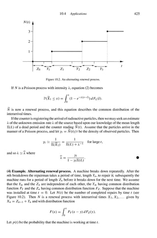
![426 10.4 Renewals
(5) Lemma. We have that
p(t) = 1 - Fz(t) + fotp(t - x) dF(x)
and hence
p(t) = 1 - Fz(t) + fo1 - Fz(t - x)] dm(x)
where m is the renewaljunction ofN.
Proof. The probability that the machine is on at time t satisfies
p(t) = lP'(on at t) = lP'(Zo > t) + lP'(on at t, Zo ::::: t)
= lP'(Zo > t) + E[lP'(on at t, ZO ::::: t I Xl)]
= lP'(Zo > t) + fotlP'(on at t I Xl = x) dF(x)
since lP'(on at t, ZO ::::: t I Xl > t) = O
= lP'(Zo > t) + fotp(t - x) dF(x).
Now use Theorem (10.1.1 1). •
(6) Corollary. If Xl is not arithmetic then p(t) -+ (1 + p)-l as t -+ 00, where p
E(Y)/E(Z) is the ratio ofthe mean lengths ofa typical repairperiod and a typical working
period.
Proof. Use the key renewal theorem (10.2.7). • •
(7) Example. Superposition of renewal processes. Suppose that a room is illuminated by
two lights, the bulbs of which fail independently of each other. On failure, they are replaced
immediately. Let Nl and N2 be the renewal processes describing the occurrences of bulb
failures in the first and second lights respectively, and suppose that these are independent
processes with the same interarrival time distribution function F. Let N be the superposition
of these two processes; that is, N(t) = Nl (t) + N2(t) is the total number of failures by time
t. In general N is not a renewal process. Let us assume for the sake of simplicity that the
interarrival times of Nl and N2 are not arithmetic.
(8) Theorem. N is a renewalprocess ifand only ifNt and N2 are Poisson processes.
Proof. It is easy to see that N is a Poisson process with intensitx 2A whenever Nl and N2
are Poisson processes with intensity A. Conversely, suppose that N is a renewal process, and
write {Xn(1)}, {Xn(2)}, and {Xn} for the interarrival times of Nl , N2, and N respectively.
Clearly Xl = min{Xl (1), Xl (2)}, and so the distribution function F of Xl satisfies
(9) 1 - F(Y) = [1 - F(y)]2.
Let El (t), E2(t), and E(t) denote the excess lifetimes of Nt , N2, and N respectively at time
t. Clearly, E(t) = min{Et (t), E2(t)}, and so
� 2
lP'(E(t) > y) = lP'(Et(t) > y) .](https://image.slidesharecdn.com/grimmettstirzaker-probabilityandrandomprocessesthirded2001-220507085451-bb31ac14/85/Grimmett-Stirzaker-Probability-and-Random-Processes-Third-Ed-2001-pdf-437-320.jpg)
![10.4 Applications
Let t --+ 00 and use Theorem (10.3.5) to obtain
(10) �ioo[1 - F(x)] dx = :2 (iOO[1 - F(x)] dxr
where /1 = lE(XI) and /1 = lE(XI (1)). Differentiate (10) and use (9) to obtain
1 � 2
100
;::; [1 - F(y)] = 2[1 - F(y)] [1 - F(x)] dx
/1 /1 y
1 2
= ;::;[1 - F(y)]
/1
(this step needs furtherjustification if F is not continuous). Thus
1 - F(y) = � [1 - F(x)] dx
2�
100
/1 y
which is an integral equation with solution
( 2/1 )
F(y) = 1 - exp -
/12 Y .
427
• •
(11) Example. Delayed renewal process. The Markov chain of Example (8.3.2) indicates
that it is sometimes appropriate to allow the first interarrival time Xl to have a distribution
which differs from the shared distribution of X2, X3, . . . .
(12) Definition. Let XI , X2, . . . be independentpositive variables such that X2, X3, . .. have
the same distribution. Let
n
To = 0, Tn = L Xi, Nd(t) = max{n : Tn ::::: t}.
I
Then Nd is called a delayed (or modified) renewal process.
Another example of a delayed renewal process is provided by a variation of the Type 1
counter of (1) with particles arriving in the manner of a Poisson process. It was convenient
there to assume thatthelife ofthe counterbegan with a dead period in orderthatthe process N
of detections be a renewal process. In the absence of this assumption N is a delayed renewal
process. The theory of delayed renewal processes is very similar to that of ordinary renewal
processes and we do not explore it in detail. The renewal equation (10.1.9) becomes
where Fd is the distribution function of X1 and m is the renewal function of an ordinary
renewal process N whose interarrival times are X2, X3, . . . . It is left to the reader to check
that
(13)](https://image.slidesharecdn.com/grimmettstirzaker-probabilityandrandomprocessesthirded2001-220507085451-bb31ac14/85/Grimmett-Stirzaker-Probability-and-Random-Processes-Third-Ed-2001-pdf-438-320.jpg)
![428 10.4 Renewals
and
00
(14) md(t) = L pf(t)
k=l
where pf is the distribution function of Tk = Xl + X2 + . . . + Xk and P is the shared
distribution function of X2, X3, . . . .
With our knowledge of the properties of m, it is not too hard to show that md satisfies the
renewal theorems. Write J-i for lE(X2).
(15) Theorem. We have that:
1 1
(a) -md(t) -+ - as t -+ 00.
t J-i
(b) IfX2 is not arithmetic then
(16)
h
md(t + h) - md(t) -+ - as t -+ 00 for any h.
J-i
IfX2 is arithmetic with span A then (16) remains true whenever h is a multiple ofA.
There is an important special case for the distribution function pd.
(17) Theorem. The process Nd has stationary increments ifand only if
(18)
1 lnY
pd(y) = _ [1 - P(x)] dx.
J-i 0
If pd is given by (1 8), then Nd is called a stationary (or equilibrium) renewalprocess. We
should recognize (18) as the asymptotic distribution (10.3.5) of the excess lifetime of the
ordinary renewal process N. So the result of (17) is no surprise since Nd starts off with this
'equilibrium' distribution. We shall see that in this case md(t) = t/J-i for all t � o.
Proof of (17). Suppose that Nd has stationary increments. Then
md(s + t) = lE([Nd(s + t) - Nd(s)] + Nd(s»)
= lE(Nd(t» + lE(Nd(s»
= md(t) + md(s).
By monotonicity, md(t) = ct for some c > O. Substitute into (13) to obtain
and let t -+ 00 to obtain c = 1/J-i.
Conversely, suppose that pd is given by (18). Substitute (18) into (13) and use the method
of Lap1ace-Stie1tjes transforms to deduce that
(19)](https://image.slidesharecdn.com/grimmettstirzaker-probabilityandrandomprocessesthirded2001-220507085451-bb31ac14/85/Grimmett-Stirzaker-Probability-and-Random-Processes-Third-Ed-2001-pdf-439-320.jpg)
![10.4 Applications 429
Now, Nd has stationary increments if and only ifthe distribution of Ed(t), the excess lifetime
of Nd at t, does not depend on t. But
00
lP'(Ed(t) > y) = LlP'(Ed(t) > y, Nd(t) = k)
k=O
= lP'(Ed(t) > y, Nd(t) = 0)
+ f t lP'(Ed(t) > y, Nd(t) = k I Tk = x) dFf(x)
k=! Jo
= 1 - Fd(t + y) + 101 - F(t + y - X)] d(�Ff(x))
= 1 - Fd(t + y) + lot[1 - F(t + y - x)] dmd(x)
from (14). Now substitute (18) and (19) into this equation to obtain the result. • •
(20) Example. Markov chains. Let Y = {Yn : n � O} be a discrete-time Markov chain with
countable state space S. At last we are able to prove the ergodic theorem (6.4.21) for Y, as
a consequence of the renewal theorem (16). Suppose that Yo = i and let j be an aperiodic
state. We can suppose that j is persistent, since the result follows from Corollary (6.2.5) if j
is transient. Observe the sequence of visits of Y to the state j. That is, let
To = 0, Tn+! = min{k > Tn : Yk = j} for n � O.
TI may equal +00; actually lP'(T! < (0) = iij . Conditional on the event {Tl < oo}, the
inter-visit times
Xn = Tn - Tn-l for n � 2
are independent and identically distributed; following Example (8.3.2), Nd(t) = max{n :
Tn ::s t} defines a delayed renewal process with a renewal function md(t) = L�=l Pij (n) for
integral t. Now, adapt (16) to deal with the possibility that the first interarrival time Xl = T
equals infinity, to obtain
d d iij
Pij (n) = m (n) - m (n - 1) -+ - as n -+ 00
J-Lj
where J-Lj is the mean recurrence time of j. •
(21) Example. Sketch proof of the renewal theorem. There is an elegant proof of the
renewal theorem (10.2.5) which proceeds by coupling the renewal process Nto an independent
delayedrenewal process Nd; here is a sketch of the method. Let N be a renewal process with
interarrival times {Xn} and interarrival timedistributionfunction F with mean J-L. We suppose
that F is non-arithmetic; the proof in the arithmetic case is easier. Let Nd be a stationary
renewal process (see (17)) with interarrival times {Yn), where Y has distribution function
1 loY
Fd(y) = _ [l - F(x)] dx
J-L 0](https://image.slidesharecdn.com/grimmettstirzaker-probabilityandrandomprocessesthirded2001-220507085451-bb31ac14/85/Grimmett-Stirzaker-Probability-and-Random-Processes-Third-Ed-2001-pdf-440-320.jpg)
![430 10.4 Renewals
and Y2, Y3, . . . have distribution function F; suppose further that the Xi are independent of
the Yi. The idea of the proof is as follows.
(a) For any E > 0, there must exist an arrival time Ta = 'Lf Xi of N and an arrival time
T; = 'L� Yi of Nd such that I Ta - T;I < E.
(b) If we replace Xa+l , Xa+2, . . . by Yb+l , Yb+2, . . . in the construction of N, then the
distributional properties of N are unchanged since all these variables are identically
distributed.
(c) But the Yi are the interarrival times ofa stationaryrenewal process, forwhich (19)holds;
this implies that md(t + h) - md(t) = hi11 for all t, h. However, met) and md(t) are
nearly the same for large t, by the previous remarks, and so m(t + h) - m(t) c::=. hi11 for
large t.
The details of the proof are slightly too difficult for inclusion here (see Lindvall 1977). •
(22) Example. Age-dependent branching process. Consider the branching process Z(t)
of Section 5.5 in which each individual lives for a random length oftime before splitting into
its offspring. We have seen that the expected number met) = JE(Z(t)) of individuals alive at
time t satisfies the integral equation (5.5.4):
(23) met) = v lot
met - x) dFT(X) + ['0 dFT(X)
where FT is the distribution function ofa typical lifetime and v is the mean number ofoffspring
of an individual; we assume for simplicity that FT is continuous. We have changed some of
the notation of (5.5.4) for obvious reasons. Equation (23) reminds us of the renewal-type
equation (10.1.10) but the factor v must be assimilated before the solution can be found using
the method of Theorem (10. 1 . 1 1). This presents few difficulties in the supercritical case. If
v > 1, there exists a unique {3 > 0 such that
F;({3) = ('0 e-fJx dFT(X) = �;
Jo v
this holds because the Lap1ace-Stieltjes transform F;(e) is a strictly decreasing continuous
function of e with
F;(O) = 1, F;(e) -+ 0 as e -+ 00.
Now, with this choice of {3, define
P(t) = v lot
e-fJx dFT(X), get) = e-fJtm(t).
Multiply through (23) by e-fJt to obtain
(24) get) = h(t) + lot
get - x) dP(x)
where
h(t) = e-fJt[1 - FT (t)];
(24) has the same general form as (10.1.10), since our choice for {3 ensures that P is the
distribution function of a positive random variable. The behaviour of get) for large t may be
found by applying Theorem (10.1.11) and the key renewal theorem (10.2.7). •](https://image.slidesharecdn.com/grimmettstirzaker-probabilityandrandomprocessesthirded2001-220507085451-bb31ac14/85/Grimmett-Stirzaker-Probability-and-Random-Processes-Third-Ed-2001-pdf-441-320.jpg)

![10.5 Renewal-rewardprocesses 433
(8) Example. A vital component of an aeroplane is replaced at a cost b whenever it reaches
the given age A. If it fails earlier, the cost of replacement is a. The distribution function of
the usual lifetime of a componentofthis type is F, which we assume to have density function
f. At what rate does the cost of replacing the component accrue?
Let Xl , X2, . . . be the runtimes of the component and its replacements. The Xi may be
assumed independent with common distribution function
H(x) = { ;(X) if x < A,
if x � A.
By Lemma (4.3.4), the mean of the Xi is
lEX = foA
[1 - F(x)] dx.
The cost of replacing a component having runtime X is
{ a if X < A,
S(X) =
b if X � A,
whence lES = aF(A) + b[1 - F(A)].
(9)
By the renewal-reward theorem (1), the asymptotic cost per unit time is
lES aF(A) + b[1 - F(A)]
lEX foA[1 - F(x)] dx
One may choose A to minimize this expression. •
We give two major applications of the renewal-reward theorem, of which the first is to
passage times of Markov chains. Let X = {X(t) : t � O} be an irreducible Markov chain in
continuous time on the countable state space S, with transition semigroup {Pt} and generator
G = (gij). For simplicity we assume that X is the minimal process associated with its jump
chain Z, as discussed prior to Theorem (6.9.24). Let U = inf{t : X(t) =1= X(O)} be the first
'holding time' ofthe chain, and define the 'first passage time' of the state i by Fi = inf{t >
U : X(t) = i}. We define the mean recurrence time of i by JLi = lE(Fi I X(O) = i). In
avoid to avoid a triviality, we assume lSI � 2, implying by the irreducibility of the chain that
gi = -gii > 0 for each i.
(10) Theorem. Assume the above conditions, and let X(0) = i. IfJLi < 00, theproportion
oftime spent in state i, and the expectation ofthis amount, satisfy, as t -+ 00,
(11)
(12)
I 1t a.s. 1
- I{x(s)=i} ds ---+ -- ,
t 0 JLigi
I 1t 1
- Pii(S) ds -+ -- .
t 0 JLigi
We note from Exercise (6.9. 1 1b) that the limit in ( 1 1 ) and (12) is the stationary distribution
ofthe chain.](https://image.slidesharecdn.com/grimmettstirzaker-probabilityandrandomprocessesthirded2001-220507085451-bb31ac14/85/Grimmett-Stirzaker-Probability-and-Random-Processes-Third-Ed-2001-pdf-444-320.jpg)
![436 10.5 Renewals
(20) Example. Cars arrive at a car wash in the manner of a Poisson process with rate v.
They wait in a line, while the car at the head of the line is washed by the unique car-wash
machine. There is space in the line for exactly K cars, including any car currently being
washed, and, when the line is full, arriving cars leave and never return. The wash times of
cars are independent random variables with distribution function F and mean ().
Let Pi denote the proportion of time that there are exactly i cars in the line, including any
car being washed. Since the queue length is not a Markov chain (unless wash times are expo
nentially distributed), one should not talk of the system being 'in equilibrium' . Nevertheless,
using renewal theory, one may see that there exists an asymptotic proportion Pi of time.
We shall apply Little's theorem to the smaller system comprising the location at the head
of the line, that is, the car-wash machine itself. We take as regeneration points the times at
which cars depart from the machine leaving the line empty.
The 'long run average queue length' is L = 1 -PO, being the proportion of time that the
machine is in use. The 'long run rate ofarrival' A is the rate at which cars enter this subsystem,
and this equals the rate at which cars join the line. Since an arriving car joins the line with
probability 1 -PK,and since cars arrive in the manner of a Poisson process with parameter
v , we deduce that A = v (1 -PK). Finally, the 'long run average waiting time' Wis the mean
time taken by the machine to wash a car, so that W = ().
We have by Little's theorem (18) that L = AW which is to say that 1 -PO= v (1 -PK)().
This equation may be interpreted in terms of the cost of running the machine, which is
proportional to 1 -PO,and the disappointment of customers who arrive to find the line full,
which is proportional to vPK. •
Exercises for Section 1 0.5
1. If X(t) is an irreducible persistent non-null Markov chain, and u(·) is a bounded function on the
integers, show that
� r u(X(s» ds � L 7riu(i),
t Jo iES
where 1C is the stationary distribution of X(t).
2. Let M(t) be an alternating renewal process, with interarrival pairs {Xr, Yr : r :::: I }. Show that
I
r a.s. lEXl
t
Jo
I{M(s) is even} ds -----+
lEX1 + lEY!
as t -+ 00.
3. Let C(s) be the current lifetime (or age) of a renewal process N(t) with a typical interarrival time
X. Show that
� r C(s) ds �
lE(X2) as t -+ 00.
t Jo 2lE(X)
Find the corresponding limit for the excess lifetime.
4. Let j and k be distinct states of an irreducible discrete-time Markov chain X with stationary
distribution 1C. Show that
1/7rk
peT· < Tk I Xo =k) = ----------
J
lE(1j I Xo =k) + lE(Tk I Xo =j)
where Ti =min{n :::: I : Xn = i} is the first passage time to the state i. [Hint: Consider the times of
return to j having made an intermediate visit to k.]](https://image.slidesharecdn.com/grimmettstirzaker-probabilityandrandomprocessesthirded2001-220507085451-bb31ac14/85/Grimmett-Stirzaker-Probability-and-Random-Processes-Third-Ed-2001-pdf-447-320.jpg)
![438 10.6 Renewals
Invert this Laplace-Stieltjes transform formally to obtain
t 0-2 - J-t2
m(t) = - + 2 + 0(1) as t --+ oo.
J-t 2J-t
Prove this rigorously by showing that
t
lo
t
met) = - - FE (t) + [1 - FE (t - x)] dm(x),
J-t 0
where FE is the asymptotic distribution function of the excess lifetime (see Exercise (l0.3.3)), and
applying the key renewal theorem. Compare the result with the renewal theorems.
12. Show that the renewal function md of a delayed renewal process satisfies
where m is the renewal function of the renewal process with interarrival times X2, X3, . . . .
13. Let m(t) be the mean number ofliving individuals at time t in an age-dependent branching process
with exponential lifetimes, parameter 'A, and mean family size v (> 1). Prove that m(t) = Ie(v-l)At
where I is the number of initial members.
14. Alternating renewal process. The interarrival times of this process are Zo , YI , Z] , Y2, . . . ,
where the Yi and Zj are independent with respective common moment generating functions My and
Mz. Let pet) be the probability that the epoch t of time lies in an interval of type Z. Show that the
Laplace-Stieltjes transform p* of p satisfies
p*(B) =
-,--_l
---,-
-------,
M
--=
z
=-
(
'::-
-
::-
B
'-,-
) -----:-:-
1 - My (-B)Mz(-B)
15. Type 2 counters. Particles are detected by a Type 2 counter of the following sort. The incoming
particles constitute a Poisson process with intensity 'A. The jth particle locks the counter for a length
Yj of time, and annuls any after-effect of its predecessors. Suppose that Yl , Y2, . , . are independent of
each other and of the Poisson process, each having distribution function G. The counter is unlocked
at time O.
Let L be the (maximal) length of the first interval of time during which the counter is locked.
Show that H(t) = JP'(L > t) satisfies
H(t) = e-At[1 - G(t)] + lH(t - x)[l - G(x)]'Ae-AX dx.
Solve for H in terms of G, and evaluate the ensuing expression in the case G(x) = 1 - e-!-'x where
J-t > O.](https://image.slidesharecdn.com/grimmettstirzaker-probabilityandrandomprocessesthirded2001-220507085451-bb31ac14/85/Grimmett-Stirzaker-Probability-and-Random-Processes-Third-Ed-2001-pdf-449-320.jpg)
![442 1 1 .2 Queues
the queue length grows beyond all bounds with probability 1 ; in the former case, the queue
attains an equilibrium as t -+ 00. It is a noteworthy conclusion that the threshold between
instability and stability depends on the mean values of Fx and Fs alone.
11.2 MIMIl
The queue M(A)/M(JL)/l is very special in that Q is a continuous-time Markov chain. Fur
thermore, reference to (6. 1 1 . 1) reminds us that Q is a birth-death process with birth and death
rates given by
An = A for all n,
_ { JL if n 2: 1,
JLn - 0 if n = o.
The probabilities Pn(t) = lP'(Q(t) = n) satisfy the Kolmogorov forward equations in the
usual way:
(1)
(2)
dPn
dt = APn-I(t) - (A +JL)Pn(t) +JLPn+I(t) for n 2: 1 ,
dpo
dt = -APO(t) +JLPI(t),
subject to the boundary conditions Pn(O) = Dan, the Kronecker delta. It is slightly tricky to
solve these equations, but routine methods provide the answer after some manipulation. There
are at least two possible routes: either use generating functions or use Laplace transforms with
respect to t. We proceed in the latter way here, and define the Laplace transformt of Pn by
(3) Theorem. We have that Pn(8) = 8-1[ 1 - a(8)]a(8)n where
(4)
(A +JL +8) - J(A +JL +8)2 - 4AJL
a�) = .
2JL
The actual probabilities Pn(t) can be deduced in terms of Bessel functions. It turns out
that pn(t) = Kn(t) - Kn+I(t) where
and In(x) is a modified Bessel function (see Feller 1971, p. 482), defined to be the coefficient
of zn in the power series expansion of exp[!x (z + Z-I)]. See Exercise (5) for another
representation of Pn(t).
tDo not confuse Pn with the Laplace-Stieltjes transform p:; CO) = Jooo e-et dpn (t).](https://image.slidesharecdn.com/grimmettstirzaker-probabilityandrandomprocessesthirded2001-220507085451-bb31ac14/85/Grimmett-Stirzaker-Probability-and-Random-Processes-Third-Ed-2001-pdf-453-320.jpg)
![1 1 .2 MlMI1
Proof. Transfonn (1) and (2) to obtain
(5)
(6)
I'-Pn+! -(A+I'-+B)Pn+APn-1 = 0 for n � 1,
I'-PI - (A+B)po = - 1,
where we have used the fact (see equation (14) of Appendix I) that
1000 -8t dPn �
e - dt = BPn -DOn,
o dt for all n.
443
Equation (5) is an ordinary difference equation, and standard techniques (see Appendix I)
show that it has a unique solution which is bounded as B � 00 and which is given by
(7)
where a is given by (4). Substitute (7) into (6) to deduce that po(B) = [1 - a(B)]jB and the
proof is complete. Alternatively, po(B) may be calculated from the fact that LnPn(t) = 1,
implying that LnPn(B) = B-1 . •
The asymptotic behaviour of Q(t) as t � 00 is deducible from (3),but more direct methods
yield the answer more quickly. Remember that Q is a Markov chain.
(8) Theorem. Let p = A.jI'- be the traffic intensity.
(a) Ifp <; 1, then lP'(Q(t) = n) --+ (1 - p)pn = ](n for n � 0, where Jt is the unique
stationary distribution.
(b) Ifp ::::: 1. there is no stationary distribution, and lP'(Q(t) == n) --+ °forall n.
The result is very natural. It asserts that the queue settles down into equilibrium if and
only if interarrival times exceed service times on average. We shall see later that if p > 1
then JtD(Q(t) � 00 as t � (0) = 1, whilst if p = 1 then the queue length experiences wild
oscillations with no reasonable bound on their magnitudes.
Proof. The process Q is an irreducible chain. Let us try to find a stationary distribution, as
done in greater generality at (6. 1 1.2) for birth-death chains. Let t � 00 in (1) and (2) to find
that the mass function 7C is a stationary distribution if and only if
(9)
nn+! - (1 +p)nn +pnn-I = 0 for n � 1,
nl -pno = O.
(The operation oftaking limits is justifiable by (6.9.20) and the unifonnity of Q.) The general
solution to (9) is
nn =
{ A+Bpn if p =1= 1,
A+Bn if p = 1,
where Aand B are arbitrary constants. Thus the only bounded solution to (9) with bounded
sum is
nn =
{ Bpn if p <; 1,
o ifp � 1.
Hence, if p <; 1, nn = (1 -p)pn is a stationary distribution, whilst if p � 1 then there exists
no stationary distribution. By Theorem (6.9.21), the proof is complete. •](https://image.slidesharecdn.com/grimmettstirzaker-probabilityandrandomprocessesthirded2001-220507085451-bb31ac14/85/Grimmett-Stirzaker-Probability-and-Random-Processes-Third-Ed-2001-pdf-454-320.jpg)
![1 1 .3 MlG/] 445
By applying this resultto the case when eo= A, en = 1.. +f-t for n � I , deducethatthe equilibrium
distribution of the M(A)IM(f-t)/1 queue is Vn = (1 - p)pn, n � 0, where p = 1../f-t < l.
3. Waiting time. Consider a M(A)1M(f-t)/1 queue with p = 1../f-t satisfying p < 1 , and suppose that
the number Q (O) of people in the queue at time 0 has the stationary distribution ]fn = (1 - p)pn,
n � O. Let W be the time spent by a typical new arrival before he begins his service. Show that the
distribution of W is given by lP'(W .::; x) = 1 - pe-x(I-'-J...) for x � 0, and note that lP'(W = 0) = 1 - p.
4. A box contains i red balls and j lemon balls, and they are drawn at random without replacement.
Each time a red (respectively lemon) ball is drawn, a particle doing a walk on {O, 1 , 2, . . . } moves
one step to the right (respectively left); the origin is a retaining barrier, so that leftwards steps from
the origin are suppressed. Let ]fen; i, j) be the probability that the particle ends at position n, having
started at the origin. Write down a set of difference equations for the ]fen; i, j), and deduce that
]fen; i, j) = A(n; i, j) - A(n + 1 ; i, j) for i .::; j + n
where A(n; i, j) = (�)/e!
n
).
5. Let Q be a M(A)IM(f-t)1l queue with Q(O) = O. Show that Pn (t) = lP'(Q(t) = n) satisfies
where the ]fen; i, j) are given in the previous exercise.
6. Let Q(t) be the length of an M(A)IM(f-t)11 queue at time t, and let Z = {Zn } be thejump chain
of Q. Explain how the stationary distribution of Q may be derived from that of Z, and vice versa.
7. Tandem queues. Two queues have one server each, and all service times are independent and
exponentially distributed, with parameter f-ti for queue i. Customers arrive at the first queue at the
instants of a Poisson process of rate A « min{f-t1 , f-t2 }), and on completing service immediately enter
the second queue. The queues are in equilibrium. Show that:
(a) the output of the first queue is a Poisson process with intensity A, and that the departures before
time t are independent of the length of the queue at time t,
(b) the waiting times of a given customer in the two queues are not independent.
11.3 MlG!l
MlM/1 is the only queue which is a Markov chain; the analysis of other queueing systems
requires greater ingenuity. If either interarrival times or service times are exponentially dis
tributed then the general theory of Markov chains still provides a method for studying the
queue. The reason is that, for each of these two cases, we may find a discrete-time Markov
chain which is imbedded in the continuous-timeprocess Q. We consider M/G/1 in this section,
which is dividedintothreepartsdealingwith eqUilibriumtheory, the 'waiting time' ofa typical
customer, and the length of a typical 'busy period' during which the server is continuously
occupied.
(A) Asymptotic queue length. Consider M(A)/G/I . Customers arrive in the manner of a
Poisson process with intensity A. Let Dn be the time of departure ofthe nth customer from the
system, and let Q(Dn) be the number of customers which he leaves behind him in the system
on his departure (really, we should write Q(Dn +) instead of Q(Dn) to make clear that the
departing customer is not included). Then Q(D) = { Q(Dn) : n 2: 1 } is a sequence ofrandom](https://image.slidesharecdn.com/grimmettstirzaker-probabilityandrandomprocessesthirded2001-220507085451-bb31ac14/85/Grimmett-Stirzaker-Probability-and-Random-Processes-Third-Ed-2001-pdf-456-320.jpg)
![1 1 .3 MIGI1 447
where S= Sn+l is the service time of the (n + l)th customer. Thus
as required, since, conditional on S, Un has the Poisson distribution with parameter AS.
Likewise, if i :::: 1 then
( . . ) { OJ-i+l
Pij = JE lP'(Un = ] - I + 1 I S) =
0
if j - i + I :::: 0,
if j - i + 1 < o.
•
This result enables us to observe the behaviour of the process Q = {Q(t)} by evaluating
it at the time epochs DJ , D2, . . . and using the theory of Markov chains. It is important to
note that this course of action provides reliable information about the asymptotic behaviour
of Q only because Dn --+ 00 almost surely as n --+ 00. The asymptotic behaviour of Q(D)
is described by the next theorem.
(5) Theorem. Let p = .A.E(S) be the traffic intensity.
(a) Ifp < 1, then Q(D) is ergodic with a unique stationary distribution 'If, having gener
atingjunction
" j Ms(.A.(s - 1»
G(8) = '-:-r1tjS =
(1 - p)(s - 1) S _ Ms(.A.(s _ 1» '
J
where Ms is the moment generatingfunction ofa typicalservice time.
(b) Ifp > 1, then Q(D) is transient.
(c) I
fp = 1, then QeD) is nullpersistent.
Here are some consequences of this theorem.
(6) Busy period. A busyperiod is a period of time during which the server is continuously
occupied. The length B of a typical busy period behaves similarly to the time B' between
successive visits of the chain Q(D) to the state O. Thus
if p < I then JE(B) < 00,
if p = I then JE(B) = 00,
if p > 1 then lP'(B = 00) > O.
lP'(B = 00) = 0,
See the forthcoming Theorems (17) and (18)for more details about B.
(7) Stationarity of Q. It is an immediate consequence of (5) and Theorem (6.4. 17) that
Q(D) is asymptotically stationary whenever p < 1 . In this case it can be shown that Q is
asymptotically stationary also, in thatlP'(Q(t) = n) --+ 7rnas t --+ 00. Roughly speaking, this
is because Q(t) forgets more and more about its origins as t becomes larger.
Proof of (5). The sequence Q(D) is irreducible and aperiodic. We proceed by applying
Theorems (6.4.3), (6.4. 10), and (6.4. 1 3).](https://image.slidesharecdn.com/grimmettstirzaker-probabilityandrandomprocessesthirded2001-220507085451-bb31ac14/85/Grimmett-Stirzaker-Probability-and-Random-Processes-Third-Ed-2001-pdf-458-320.jpg)
![448 1 1 .3 Queues
(a) Look for a root ofthe equation 7C = 7C PD . Any such 7C satisfies
(8)
J+I
7r) = 7r00) +L 7riO)-i+I, for j :::: O.
i=1
First, note thatif7r0 (::::0)is given, then (8)has a unique solution 7C . Furthermore, this solution
has non-negative entries. To see this, add equations (8)for j = 0, 1 , . . . , n and solve for
7rn+l to obtain
(9)
where
n
7rn+IOO = 7rOEn +L 7riEn-i+1 for n :::: 0
i=1
En = 1 - DO- 01 - . . . - On > 0 because L D) = 1 .
)
From (9), 7rn+1 :::: 0whenever 7ri :::: 0for all i ::::: n, and so
(10) 7rn :::: 0 for all n
if 7r0 :::: 0,by induction. Return to (8)to see that the generating functions
satisfy
and therefore
(11)
G(s) = L 7r)s), �(s) = L O)s),
) )
1
G(s) = 7rO�(s) +-[G(s) - 7ro]�(s)
s
G(s) =
7ro(s - l)�(s)
.
s - �(s)
The vector 7C is a stationary distribution if and only if 7r0 > 0and limst1 G(s) = 1 . Apply
L'Hopital's rule to (1 1) to discover that
7r0 = 1 - �'(1) > 0
is a necessary and sufficient condition for this to occur, and thus there exists a stationary
distribution if and only if
(12) �I(l) < 1 .
However,](https://image.slidesharecdn.com/grimmettstirzaker-probabilityandrandomprocessesthirded2001-220507085451-bb31ac14/85/Grimmett-Stirzaker-Probability-and-Random-Processes-Third-Ed-2001-pdf-459-320.jpg)
![11.5 GIGI1 455
Look for a solution of the form lTn = en for some e, and deduce that the unique stationary distribution
is given by lTj = (l - 7])7]i for j :::: 0, where 7] is the smallest positive root of the equation s =
MX (f-t(s - 1» .
2. Consider a GIM(f-t)!1 queue in equilibrium. Let 7] be the smallest positive root of the equation
x = MX (f-t(x - 1» where MX is the moment generating function of an interarrival time. Show that
the mean number of customers ahead of a new arrival is 7] (l - 7])-1 , and the mean waiting time is
7]{f-t(1 - 7])}-1 .
3. Consider D(l)IM(f-t)/1 where f-t > 1 . Show that the continuous-time queue length Q(t) does not
converge in distribution as t ---+ 00, even though the imbedded chain at the times of arrivals is ergodic.
11.5 G/G/l
If neither interarrival times nor service times are exponentially distributed then the methods
ofthe last three sections fail. This apparent setback leads us to the remarkable discovery that
queueing problems are intimately related to random walk problems. This section is divided
into two parts, one dealing with the equilibrium theory of GIGll and the other dealing with
the imbedded random walk.
(A) Asymptotic waiting time. Let Wn be the waiting time of the nth customer. There is a
useful relationship between Wn and Wn+l in terms of the service time Sn of the nth customer
and the length Xn+l of time between the nth and the (n + l)th arrivals.
(1) Theorem. Lindley's equation. We have that
Wn+l = max{O, Wn + Sn - Xn+d·
Proof. The nth customer is in the system for a length Wn + Sn of time. If Xn+l > Wn + Sn
then the queue is empty at the (n + l)th arrival, and so Wn+l = O. If Xn+l ::::; Wn + Sn then
the (n + 1 )th customer arrives while the nth is still present, but only waits for a period of
length Wn + Sn - Xn+l before the previous customer leaves. •
We shall see that Lindley's equation implies that the distribution functions
ofthe Wn convergeas n ---+ (Xl to some limit function F(x). Of course, F need not be a proper
distribution function; indeed, it is intuitively clear thatthe queue settles down into equilibrium
if and only if F is a distribution function which is not defective.
(2) Theorem. Let Fn(x) = JP'(Wn ::::; x). Then
ifx < 0,
ifx 2: 0,
where GisthedistributionfunctionofUn = Sn -Xn+l. Thusthe limit F(x) = limn---+oo Fn(x)
exists.](https://image.slidesharecdn.com/grimmettstirzaker-probabilityandrandomprocessesthirded2001-220507085451-bb31ac14/85/Grimmett-Stirzaker-Probability-and-Random-Processes-Third-Ed-2001-pdf-466-320.jpg)
![11.5 GIGI] 459
that is, L(n + 1) is the earliest epoch m of time at which :Em exceeds the walk's previous
maximum :EL(n) . The L(n) are called ladderpoints; negative ladderpoints of :E are defined
similarly as the epochs at which :E attains new minimum values. The result of (4)amounts to
the assertion that
{ 0 if lE(U) < 0,
lP'(there exist infinitely many ladder points) =
1 if lE(U) > O.
The total number of ladder points is given by the next lemma.
(12) Lemma. Let TJ = lP'(:En > 0for some n � 1)be theprobability that at least one ladder
point exists. The total number A ofladderpoints has massfunction
lP'(A = I) = (1 - TJ)TJI for I � o.
Proof. The process :E is a discrete-time Markov chain. Thus
lP'(A � I + 1 I A � I) = TJ
since the path of the walk after the Ith ladder point is a copy of :E itself. •
Thus the queue is stable if TJ < 1,in which case the maximum W' of :E is related to the
height of a typical ladder point. Let
be the difference in the displacements of the walk at the (j - l)th and jth ladder points.
Conditional on the value of A, {Yj : 1 ::s j ::s A} is a collection of independent identically
distributed variables, by the Markovproperty. Furthermore,
(13)
A
W'= :EL(A) = L Yj;
j=l
this leads to the next lemma, relating the waiting time distribution to the distribution of a
typical Yj.
(14) Lemma. Ifthetrafficintensityp satisfiesp < 1,theequilibriumwaitingtimedistribution
has momentgeneratingfunction
I - TJ
Mw(s) = ----
1 -TJMy(s)
where My is the moment generatingfunction ofY.
Proof. We have that p < 1 if and only if TJ < 1. Use (13)and (5.1.25)to find that
Now use the result of Lemma (12). •](https://image.slidesharecdn.com/grimmettstirzaker-probabilityandrandomprocessesthirded2001-220507085451-bb31ac14/85/Grimmett-Stirzaker-Probability-and-Random-Processes-Third-Ed-2001-pdf-470-320.jpg)
![11.5 GIGI1 461
Proof. Let Q have interarrival times {Xn}and service times {Sn}; I; has jumps of size Un =
Sn -Xn+! (n :::: 1). The reflected walk -I; , which is obtained by reflecting I; in the x-axis,
hasjumps ofsize -Un = Xn+!-Sn(n :::: 1)(see Section 3.10for more details ofthe reflection
principle). Write {S�}and {X�}for the interarrival and service times of Qd; I;d has jumps of
size U�= X� -S�+! (n :::: 1), which have the same distribution as thejumps of - I; . •
This leads to a corollary.
(19) Theorem. The height Y ofthefirst ladderpoint of I; has the same distribution as the
length Id ofa typical idleperiod in the dual queue.
Proof. From (15), -Id is the heightofthe first ladderpointof -I;d, whichby (18)is distributed
as the height Y of the first ladder point of I; . •
Here is an example of an application of these facts.
(20) Theorem. Let Q be a stable queueingprocess with dualprocess Qct. Let Wbe a typical
equilibrium waiting time of Q and Id a typical idleperiod of Qd. Their moment generating
junctions are relatedby
where 1'/ = P(W > 0).
Proof. Use (14)and (19).
1 - 1'/
Mw(s) = ----
1 - 1'/M1d (s)
•
An application of this result is given in Exercise (2). Another application is a second
derivation of the equilibrium waiting time distribution (11.4.12)of GIM/I ; just remark that
the dual of GIMIl is M/G/l , and that idle periods of M/G/I are exponentially distributed
(though, of course, the server does not have many such periods if the queue is unstable).
Exercises for Section 1 1 .5
1. Show that, for a GIGII queue, the starting times of the busy periods of the server constitute a
renewal process.
2. Consider a GIM(Jl)/1 queue in equilibrium, together with the dual (unstable) M(Jl)/G/1 queue.
Show that the idle periods of the latter queue are exponentially distributed. Use the theory of duality
of queues to deduce for the former queue that: (a) the waiting-time distribution is a mixture of an
exponential distribution and an atom at zero, and (b) the equilibrium queue length is geometric.
3. Consider GIM(Jl)/1 , and let G be the distribution function of S - X where S and X are typical
(independent) service and interarrival times. Show that the Wiener-Hop!equation
F(x) = 1:00F(x- y) dG(y), x 2: 0,
for the limiting waiting-time distribution Fis satisfied by F(x) = I - I]e-/L(1-rJ)x, x 2: O. Here, I]
is the smallest positive root of the equation x= MX (Jl(x- I )), where Mx is the moment generating
function of X.](https://image.slidesharecdn.com/grimmettstirzaker-probabilityandrandomprocessesthirded2001-220507085451-bb31ac14/85/Grimmett-Stirzaker-Probability-and-Random-Processes-Third-Ed-2001-pdf-472-320.jpg)
![462 11.7 Queues
11.6 Heavy traffic
A queue settles into equilibrium if its traffic intensity p is less than 1 ; it is unstable if p > 1. It
is our shared personal experience that many queues (such as in doctors' waiting rooms and at
airport check-in desks) have a tendency to become unstable. The reason is simple: employers
do not like to see their employees idle, and so they provide only just as many servers as are
necessary to cope with the arriving customers. That is, they design the queueing system so
that p is only slightly smaller than 1; the ensuing queue is long but stable, and the server
experiences 'heavy traffic' . As p t I the equilibrium queue length Qp becomes longer and
longer, and it is interesting to ask for the rate at which Qp approaches infinity. Often it turns
out that a suitably scaled form of Qp is asymptotically exponentially distributed. We describe
this here for the M/D/1 system, leaving it to the readers to amuse themselves by finding
corresponding results for other queues. In this special case, Qp � Z/(1 - p) as p t I where
Zis an exponential variable.
(1) Theorem. Let p = Ad be the traffic intensity ofthe M(A)/D(d)/I queue, andlet Qp be
a random variable with the equilibrium queue lengthdistribution. Then (1- p) Qp converges
in distribution as p t 1 to the exponential distribution with parameter 2.
Proof. Use (11.3.5)to see that Qp has moment generating function
(2)
(1 - p)(eS - 1)
M (s) - if p < 1 .
p - exp[s - p ees - 1)] - 1
The moment generating function of (1 - p) Qp is Mp «1 - p)s), and we make the appro
priate substitution in equation (2). Now let p t 1 and use L'Hopital's rule to deduce that
Mp«1 - p)s) -+ 2/(2 - s). •
Exercise for Section 1 1 .6
1. Consider the M(A.)!M(p,)11 queue with p = A.Ip, < 1 . Let Qp be a random variable with the
equilibrium queue distribution, and show that (1 - p) Qp converges in distribution as p t 1 , the limit
distribution being exponential with parameter 1 .
11.7 Networks of queues
A customer departing from one queue may well be required to enter another. Under certain
circumstances, this customer may even, at a later stage, be required to re-enter the original
queue. Networks of queues provide natural models for many situations in real life, ranging
from the manufacture of components in complex industrial processes to an application for a
visa for travel to another country.
We make concrete our notion of a queueing network as follows. There is a finite set Sof
'stations' labelled Sl , S2, . . . , Se . At time t, station i contains Qi (t) individuals, so that the
state of the system may be represented as the vector Q(t) = ( Q ] (t), Q2(t), . . . , Qc(t». We
assume for simplicity that the process Q is Markovian, taking values in the set .N = {n =
(n1 , n2, . .. , ne) : ni = 0, 1,2, . . . for 1 ::s i ::s c} ofsequences ofnon-negative integers. The
migration of customers between stations will be described in a rather general way in order to
enable a breadth of applications.](https://image.slidesharecdn.com/grimmettstirzaker-probabilityandrandomprocessesthirded2001-220507085451-bb31ac14/85/Grimmett-Stirzaker-Probability-and-Random-Processes-Third-Ed-2001-pdf-473-320.jpg)
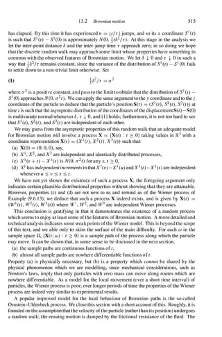
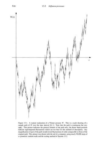
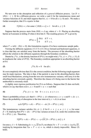
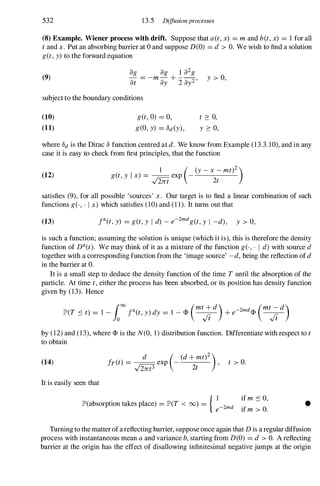
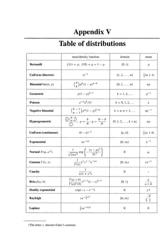
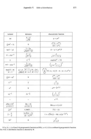
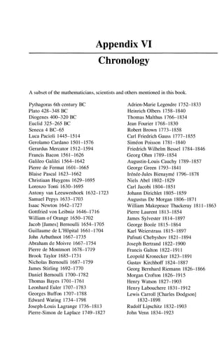


This document provides an introduction to probability theory. It defines a probability space as comprising a sample space Q of possible outcomes of an experiment, a set F of events, and a probability measure P. Q is the set of all possible outcomes, while events are subsets of Q. Examples of simple experiments with coins and dice are used to illustrate these concepts. The key concepts of conditional probability and independence are also introduced.


![[ICLR2021 (spotlight)] Benefit of deep learning with non-convex noisy gradien...](https://cdn.slidesharecdn.com/ss_thumbnails/iclr2021-210331133549-thumbnail.jpg?width=640&height=640&fit=bounds)