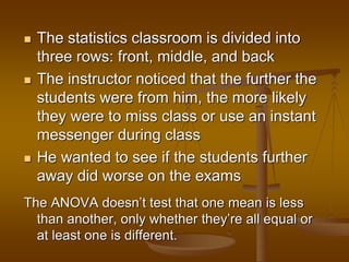
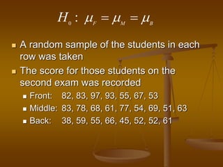
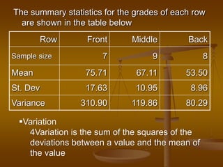
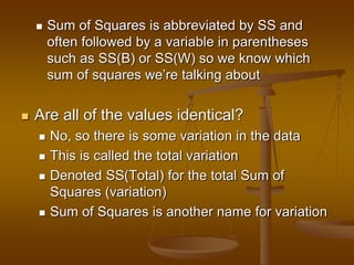
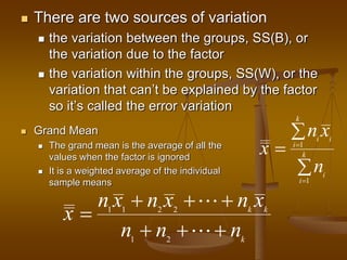
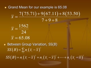
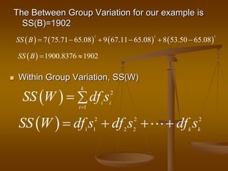
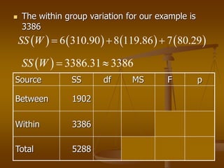
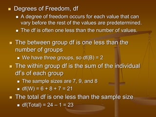
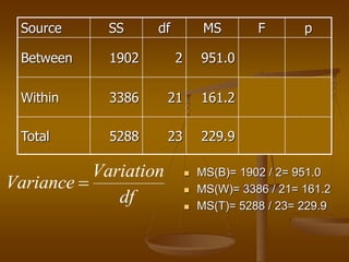
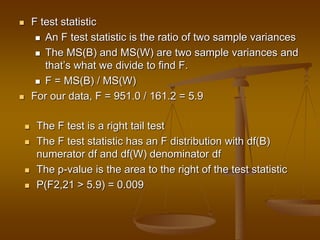
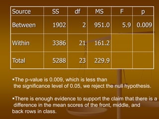
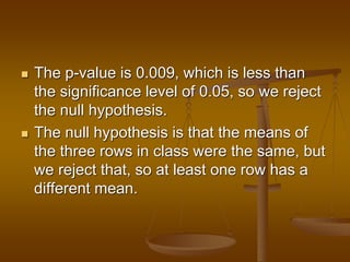
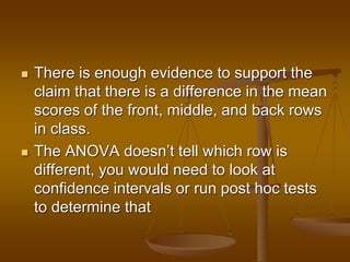
The document describes how analysis of variance (ANOVA) can be used to compare mean exam scores between students sitting in different rows (front, middle, back) of a classroom. ANOVA measures variation between and within groups. If the between-group variation is significantly greater than the within-group variation, then at least one group mean is different. The ANOVA calculation and assumptions are shown using example data. The results show the mean scores differed significantly between rows, rejecting the null hypothesis that all row means were equal.

1. BRANCH :- FOOD PROCESSING AND TECHNOLOGY
in the
Subject of Food Standard and Quality Assurance[2171401]
On the
Topic of ANOVA model [how ANOVA work?] with example
Created by :
mahesh kapadiya 150010114020
Parth patel 130010114035

2. •The analysis of variance is developed by R.A. fisher in 1920.
•If the number of sample is more than two then Z-test and T-test can not be used.
•The technique of variance analysis developed by fisher is very useful in very such
case and with it’s help it is possible to study the significance of difference of mean
values of large no. of samples at a same time.
•The variance analysis studies the significance of the difference in means by
analysing variance.
•The variances would differ only when the means are significantly different.
•The technique of the analysis of variance as developed by Fisher is capable of
Fruitful application in a variety of problems.
•Ho : Variability w/i groups = variability b/t groups.
• Ha : Variability w/i groups does not = variability b/t groups.
Introduction

3. • ANOVA measures two sources of variation in the data and compares their
relative sizes.
•variation BETWEEN groups:
for each data value look at the difference between its group mean and
the over all mean.
•variation WITHIN groups :
for each data value we look at the difference between that value and the
mean of its group.
F-STATISTICS

4. •The ANOVA F-statistic is a ratio of the Between Group
Variation divided by the Within Group Variation:
F= MSC/MSE
where, MSC: variance between the sample
and ,MSE: variance within the sample
•A large F is evidence against H0 , since it indicates that there
is more difference Between groups than within groups.

5.  The null hypothesis is that the means are all
equal
 The alternative hypothesis is that at least one
of the means is different
0 1 2 3
: k
H       
•The samples are independently drawn.
• The population are normally distributed, with common variance.
•They occur at random and independent of each other in the
groups.
•The effects of various components are additive.
Assumption in ANOVA analysis

6.  The statistics classroom is divided into
three rows: front, middle, and back
 The instructor noticed that the further the
students were from him, the more likely
they were to miss class or use an instant
messenger during class
 He wanted to see if the students further
away did worse on the exams
The ANOVA doesn’t test that one mean is less
than another, only whether they’re all equal or
at least one is different.

7. 0
: F M B
H    
 A random sample of the students in each
row was taken
 The score for those students on the
second exam was recorded
 Front: 82, 83, 97, 93, 55, 67, 53
 Middle: 83, 78, 68, 61, 77, 54, 69, 51, 63
 Back: 38, 59, 55, 66, 45, 52, 52, 61

8. The summary statistics for the grades of each row
are shown in the table below
Row Front Middle Back
Sample size 7 9 8
Mean 75.71 67.11 53.50
St. Dev 17.63 10.95 8.96
Variance 310.90 119.86 80.29
Variation
4Variation is the sum of the squares of the
deviations between a value and the mean of
the value

9.  Sum of Squares is abbreviated by SS and
often followed by a variable in parentheses
such as SS(B) or SS(W) so we know which
sum of squares we’re talking about
 Are all of the values identical?
 No, so there is some variation in the data
 This is called the total variation
 Denoted SS(Total) for the total Sum of
Squares (variation)
 Sum of Squares is another name for variation

10.  There are two sources of variation
 the variation between the groups, SS(B), or
the variation due to the factor
 the variation within the groups, SS(W), or the
variation that can’t be explained by the factor
so it’s called the error variation
 Grand Mean
 The grand mean is the average of all the
values when the factor is ignored
 It is a weighted average of the individual
sample means
1
1
k
i i
i
k
i
i
n x
x
n





1 1 2 2
1 2
k k
k
n x n x n x
x
n n n
  

  

11.  Grand Mean for our example is 65.08
     7 75.71 9 67.11 8 53.50
7 9 8
1562
24
65.08
x
x
x
 

 


 Between Group Variation, SS(B)
   
2
1
k
i i
i
SS B n x x

 
       
2 2 2
1 1 2 2 k k
SS B n x x n x x n x x      

12. The Between Group Variation for our example is
SS(B)=1902
       
2 2 2
7 75.71 65.08 9 67.11 65.08 8 53.50 65.08SS B      
  1900.8376 1902SS B  
 Within Group Variation, SS(W)
  2
1
k
i i
i
SS W df s

 
  2 2 2
1 1 2 2 k k
SS W df s df s df s   

13.  The within group variation for our example is
3386
       6 310.90 8 119.86 7 80.29SS W   
  3386.31 3386SS W  
Source SS df MS F p
Between 1902
Within 3386
Total 5288

14.  Degrees of Freedom, df
 A degree of freedom occurs for each value that can
vary before the rest of the values are predetermined.
 The df is often one less than the number of values.
 The between group df is one less than the
number of groups
 We have three groups, so df(B) = 2
 The within group df is the sum of the individual
df’s of each group
 The sample sizes are 7, 9, and 8
 df(W) = 6 + 8 + 7 = 21
 The total df is one less than the sample size
 df(Total) = 24 – 1 = 23

15. Variation
Variance
df

Source SS df MS F p
Between 1902 2 951.0
Within 3386 21 161.2
Total 5288 23 229.9
 MS(B)= 1902 / 2= 951.0
 MS(W)= 3386 / 21= 161.2
 MS(T)= 5288 / 23= 229.9

16.  F test statistic
 An F test statistic is the ratio of two sample variances
 The MS(B) and MS(W) are two sample variances and
that’s what we divide to find F.
 F = MS(B) / MS(W)
 For our data, F = 951.0 / 161.2 = 5.9
 The F test is a right tail test
 The F test statistic has an F distribution with df(B)
numerator df and df(W) denominator df
 The p-value is the area to the right of the test statistic
 P(F2,21 > 5.9) = 0.009

17. Source SS df MS F p
Between 1902 2 951.0 5.9 0.009
Within 3386 21 161.2
Total 5288 23 229.9
The p-value is 0.009, which is less than
the significance level of 0.05, we reject the null hypothesis.
There is enough evidence to support the claim that there is a
difference in the mean scores of the front, middle, and
back rows in class.

18.  The p-value is 0.009, which is less than
the significance level of 0.05, so we reject
the null hypothesis.
 The null hypothesis is that the means of
the three rows in class were the same, but
we reject that, so at least one row has a
different mean.

19.  There is enough evidence to support the
claim that there is a difference in the mean
scores of the front, middle, and back rows
in class.
 The ANOVA doesn’t tell which row is
different, you would need to look at
confidence intervals or run post hoc tests
to determine that