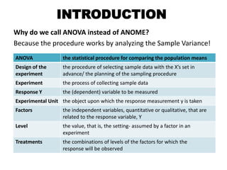
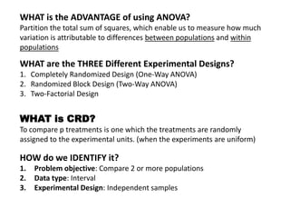
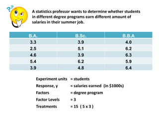
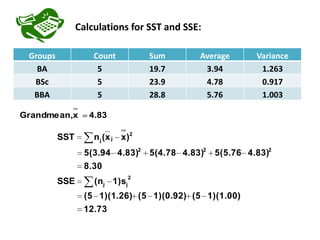
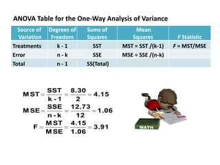
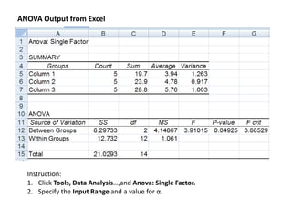
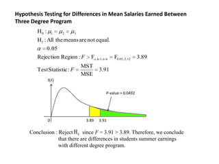
INTRODUCTION
Why do we call ANOVA instead of ANOME?
Because the procedure works by analyzing the Sample Variance!
ANOVA              the statistical procedure for comparing the population means
Design of the      the procedure of selecting sample data with the X’s set in
experiment         advance/ the planning of the sampling procedure
Experiment         the process of collecting sample data
Response Y         the (dependent) variable to be measured
Experimental Unit the object upon which the response measurement y is taken
Factors            the independent variables, quantitative or qualitative, that are
                   related to the response variable, Y
Level              the value, that is, the setting- assumed by a factor in an
                   experiment
Treatments         the combinations of levels of the factors for which the
                   response will be observed
WHAT is the ADVANTAGE of using ANOVA?
Partition the total sum of squares, which enable us to measure how much
variation is attributable to differences between populations and within
populations

WHAT are the THREE Different Experimental Designs?
1. Completely Randomized Design (One-Way ANOVA)
2. Randomized Block Design (Two-Way ANOVA)
3. Two-Factorial Design


WHAT is CRD?
To compare p treatments is one which the treatments are randomly
assigned to the experimental units. (when the experiments are uniform)

HOW do we IDENTIFY it?
1.   Problem objective: Compare 2 or more populations
2.   Data type: Interval
3.   Experimental Design: Independent samples
A statistics professor wants to determine whether students
 in different degree programs earn different amount of
 salaries in their summer job.


B.A.                    B.Sc.                    B.B.A
3.3                      3.9                      4.0
2.5                      5.1                      6.2
4.6                      3.9                      6.3
5.4                      6.2                      5.9
3.9                      4.8                      6.4

   Experiment units = students
   Response, y       = salaries earned (in $1000s)
   Factors           = degree program
   Factor Levels     =3
   Treatments        = 15 ( 5 x 3 )
Calculations for SST and SSE:

 Groups             Count            Sum    Average     Variance
   BA                5               19.7    3.94        1.263
  BSc                5               23.9    4.78        0.917
  BBA                5               28.8    5.76        1.003

Grandmean,x        4.83

          SST       n j ( x j x )2
                  5(3.94 4.83)2 5(4.78 4.83)2 5(5.76 4.83)2
                  8.30
                                2
          SSE       (nj 1)sj
                  (5 1)(1.26) (5 1)(0.92) (5 1)(1.00)
                 12.73
ANOVA Table for the One-Way Analysis of Variance
  Source of   Degrees of   Sums of          Mean
  Variation    Freedom     Squares        Squares           F Statistic
Treatments       k-1         SST       MST = SST /(k-1)   F = MST/MSE
Error            n-k         SSE       MSE = SSE /(n-k)
Total            n-1       SS(Total)


        SST           8.30
   M ST                     4.15
        k-1            2
        SSE           12.73
   M SE                      1.06
        n-k            12
        M ST          4.15
      F                     3.91
        M SE          1.06
ANOVA Output from Excel


  Instruction:
  1. Click Tools, Data Analysis…,and Anova: Single Factor.
  2. Specify the Input Range and a value for α.
Hypothesis Testing for Differences in Mean Salaries Earned Between
Three Degree Program
        H0 :       1   2     3

        H1 : All the means are not equal.
               0.05
        Rejection Region : F        F    , k -1, n - k   F0.05, 2, 12   3.89
                                 MST
        Test Statistic : F                  3.91
                                 MSE
               f(F)

                                                    P-value = 0.0492


               0                  3.89      3.91

     Conclusion : Reject H 0 since F = 3.91 > 3.89. Therefore, we conclude
                  that there are differences in students summer earnings
                  with different degree program.

Anova Presentation

  • 2.
    INTRODUCTION Why do wecall ANOVA instead of ANOME? Because the procedure works by analyzing the Sample Variance! ANOVA the statistical procedure for comparing the population means Design of the the procedure of selecting sample data with the X’s set in experiment advance/ the planning of the sampling procedure Experiment the process of collecting sample data Response Y the (dependent) variable to be measured Experimental Unit the object upon which the response measurement y is taken Factors the independent variables, quantitative or qualitative, that are related to the response variable, Y Level the value, that is, the setting- assumed by a factor in an experiment Treatments the combinations of levels of the factors for which the response will be observed
  • 3.
    WHAT is theADVANTAGE of using ANOVA? Partition the total sum of squares, which enable us to measure how much variation is attributable to differences between populations and within populations WHAT are the THREE Different Experimental Designs? 1. Completely Randomized Design (One-Way ANOVA) 2. Randomized Block Design (Two-Way ANOVA) 3. Two-Factorial Design WHAT is CRD? To compare p treatments is one which the treatments are randomly assigned to the experimental units. (when the experiments are uniform) HOW do we IDENTIFY it? 1. Problem objective: Compare 2 or more populations 2. Data type: Interval 3. Experimental Design: Independent samples
  • 4.
    A statistics professorwants to determine whether students in different degree programs earn different amount of salaries in their summer job. B.A. B.Sc. B.B.A 3.3 3.9 4.0 2.5 5.1 6.2 4.6 3.9 6.3 5.4 6.2 5.9 3.9 4.8 6.4 Experiment units = students Response, y = salaries earned (in $1000s) Factors = degree program Factor Levels =3 Treatments = 15 ( 5 x 3 )
  • 5.
    Calculations for SSTand SSE: Groups Count Sum Average Variance BA 5 19.7 3.94 1.263 BSc 5 23.9 4.78 0.917 BBA 5 28.8 5.76 1.003 Grandmean,x 4.83 SST n j ( x j x )2 5(3.94 4.83)2 5(4.78 4.83)2 5(5.76 4.83)2 8.30 2 SSE (nj 1)sj (5 1)(1.26) (5 1)(0.92) (5 1)(1.00) 12.73
  • 6.
    ANOVA Table forthe One-Way Analysis of Variance Source of Degrees of Sums of Mean Variation Freedom Squares Squares F Statistic Treatments k-1 SST MST = SST /(k-1) F = MST/MSE Error n-k SSE MSE = SSE /(n-k) Total n-1 SS(Total) SST 8.30 M ST 4.15 k-1 2 SSE 12.73 M SE 1.06 n-k 12 M ST 4.15 F 3.91 M SE 1.06
  • 7.
    ANOVA Output fromExcel Instruction: 1. Click Tools, Data Analysis…,and Anova: Single Factor. 2. Specify the Input Range and a value for α.
  • 8.
    Hypothesis Testing forDifferences in Mean Salaries Earned Between Three Degree Program H0 : 1 2 3 H1 : All the means are not equal. 0.05 Rejection Region : F F , k -1, n - k F0.05, 2, 12 3.89 MST Test Statistic : F 3.91 MSE f(F) P-value = 0.0492 0 3.89 3.91 Conclusion : Reject H 0 since F = 3.91 > 3.89. Therefore, we conclude that there are differences in students summer earnings with different degree program.