Downloaded 45 times


![Remember that…
Standard deviation (s)
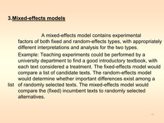
n
s = √[(Σ (xi – X)2)/(n-1)]
i = 1
In this case: Degrees of freedom (df)
df = Number of observations or groups
16](https://image.slidesharecdn.com/anova-singlefactor-140910111427-phpapp02/85/Anova-single-factor-16-320.jpg)
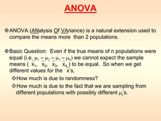
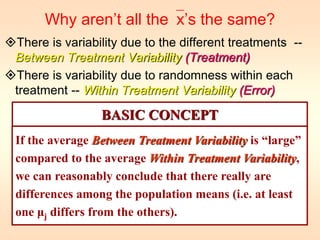
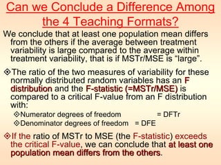

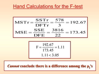


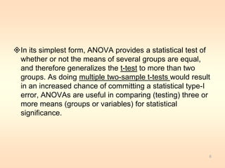
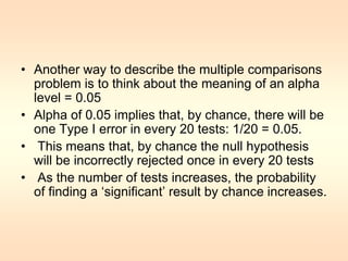
1) ANOVA is used to compare the means of more than two populations and determine if observed differences are due to chance or actual differences in the population means. 2) The document provides an example of using a one-way single factor ANOVA to analyze the effects of different teaching formats on student exam scores. 3) The ANOVA compares the between-treatment variability to the within-treatment variability using an F-test. If the between-treatment variability is significantly larger, it suggests the population means differ. In this example, the F-test showed no significant difference between the teaching formats.


