Normal Distribution.pdf

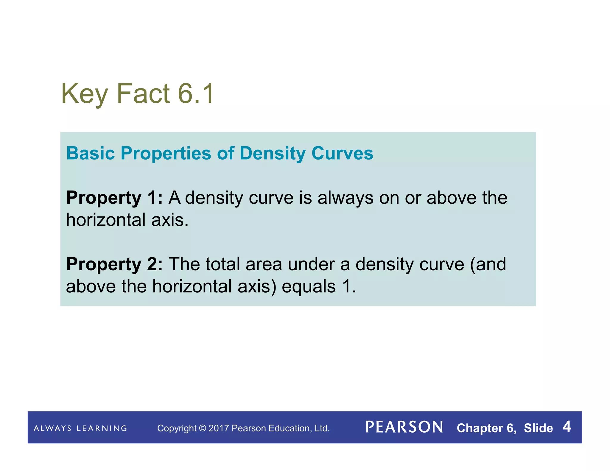
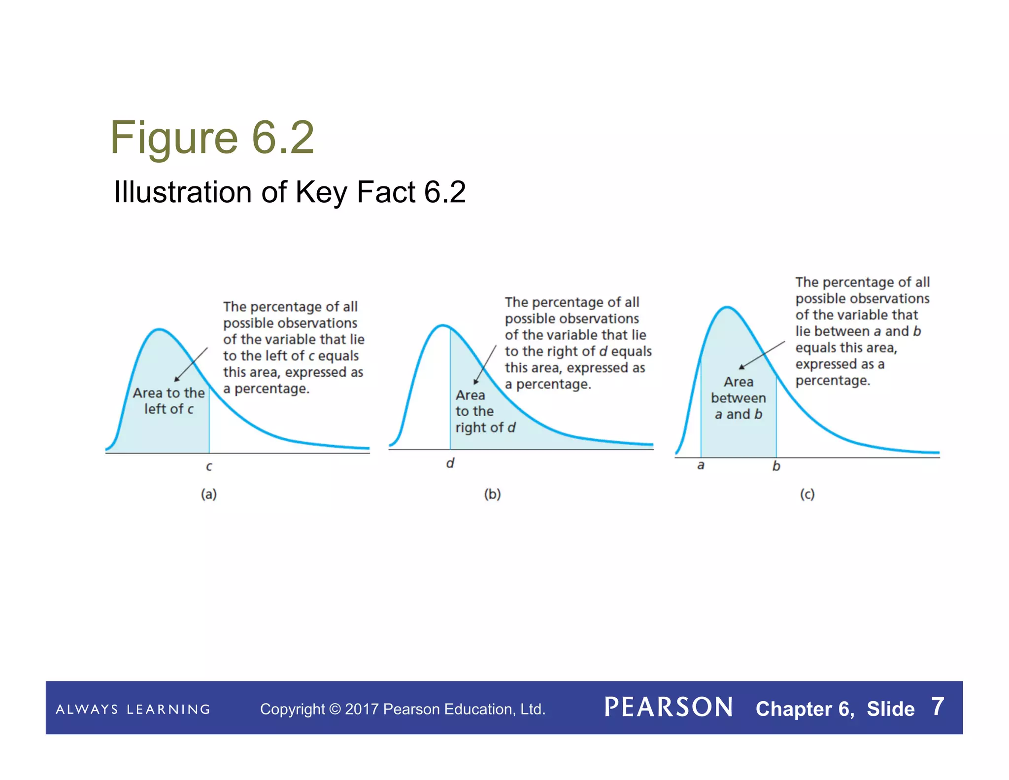
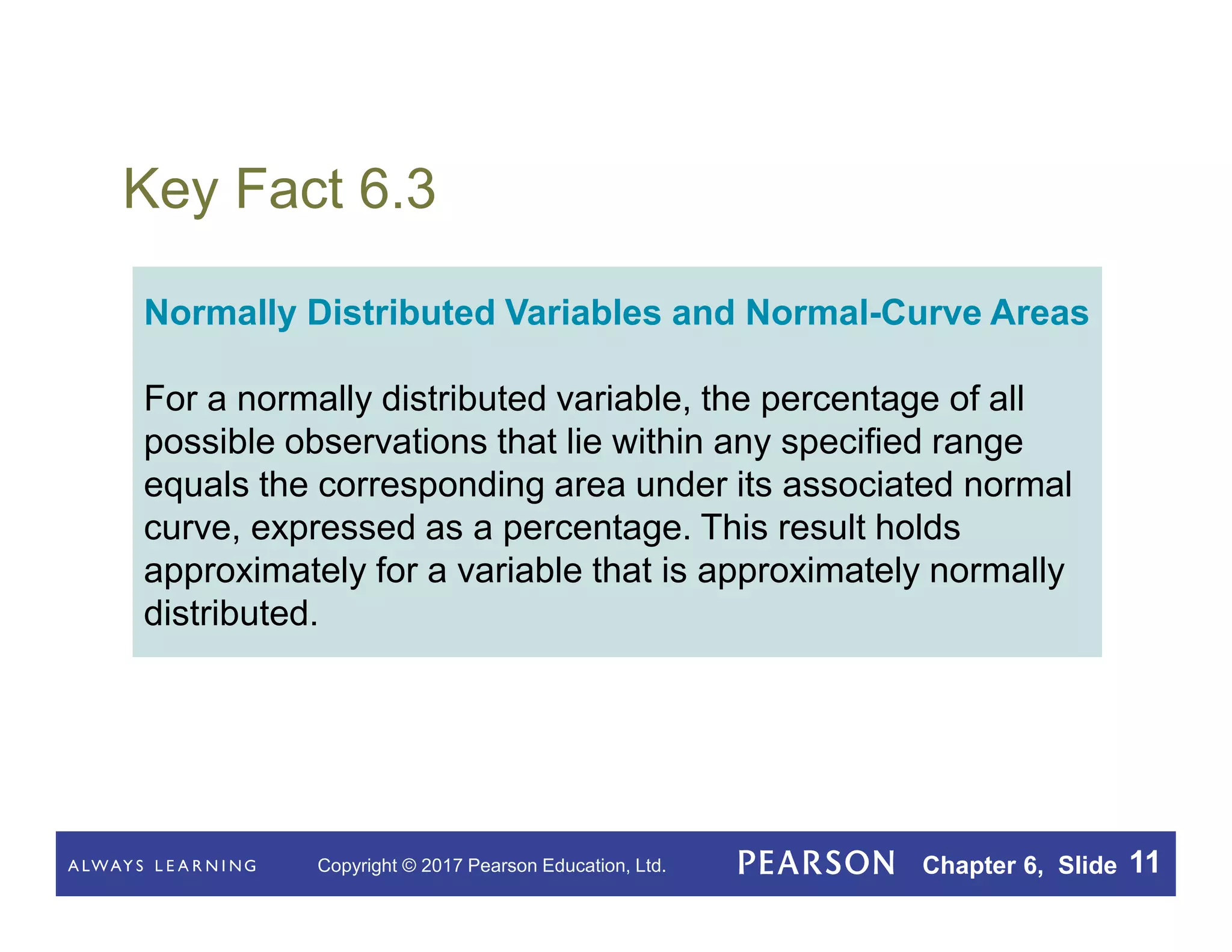
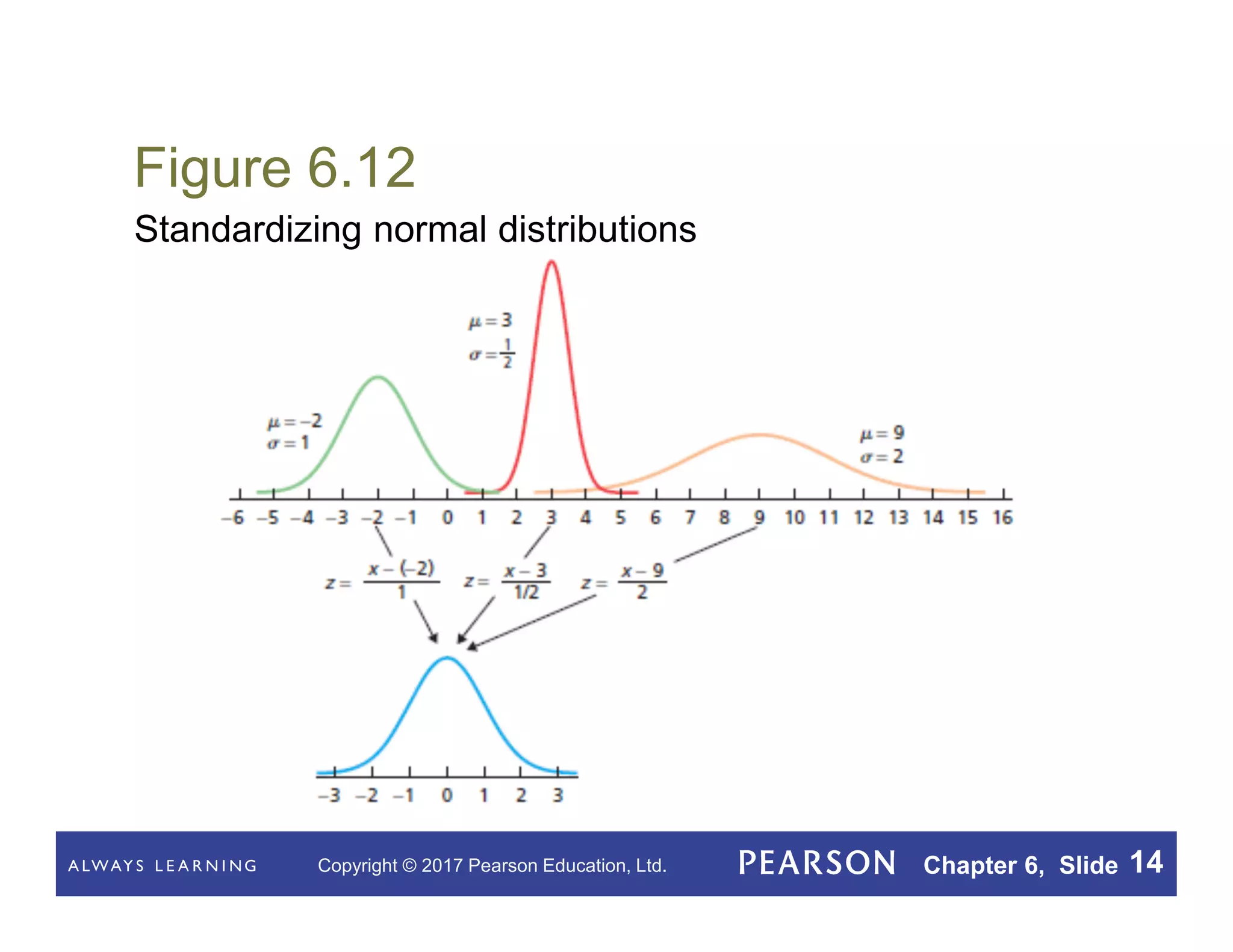
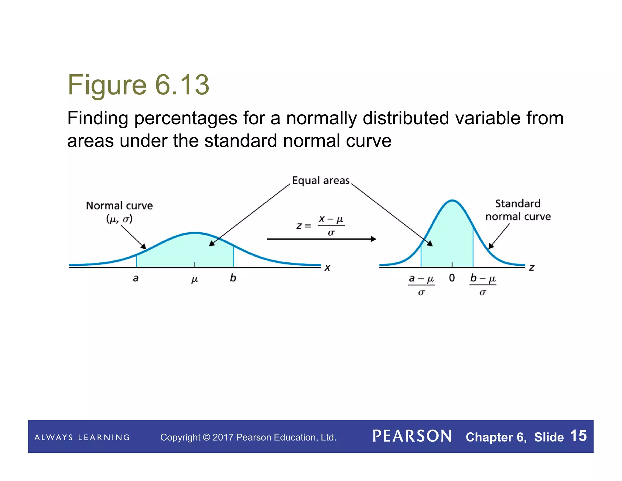
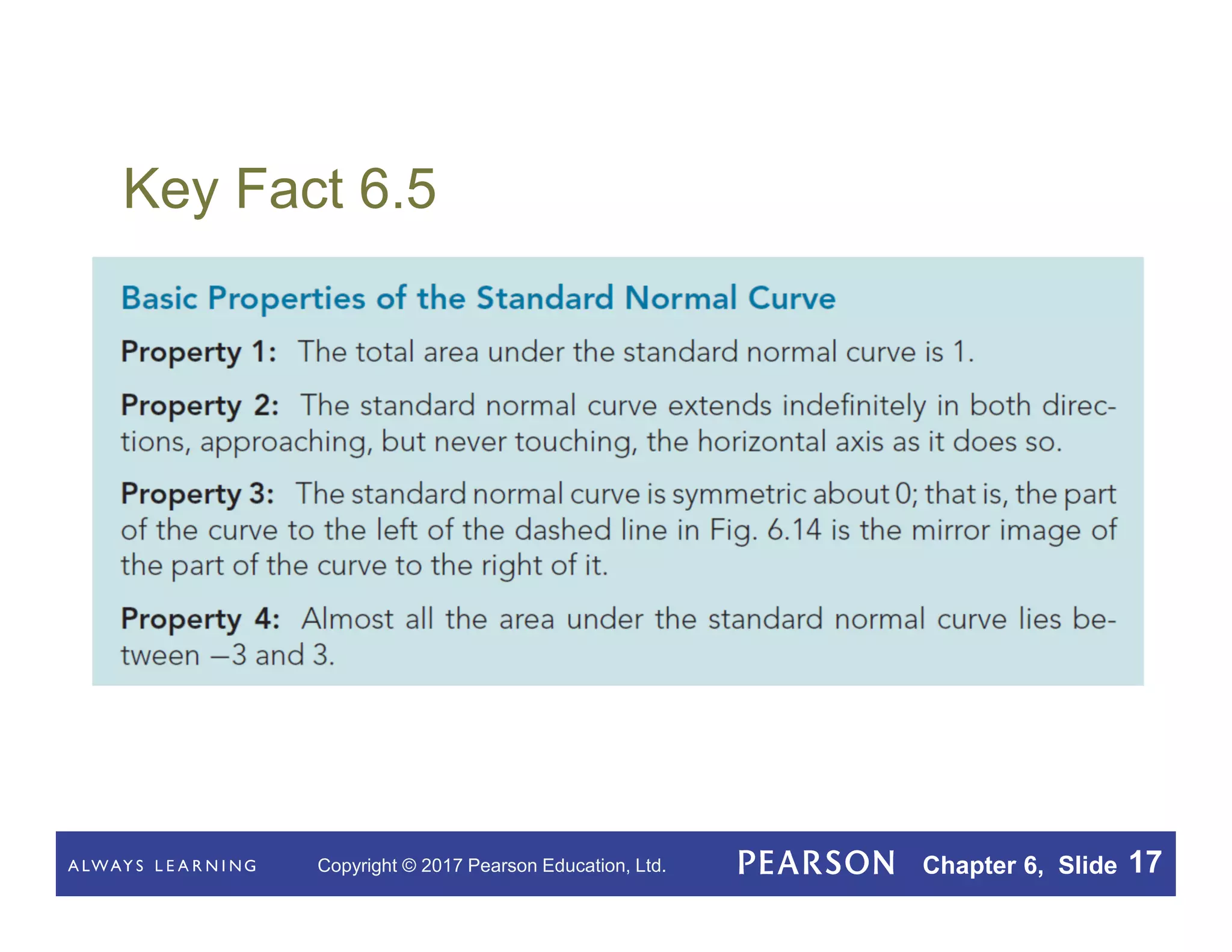
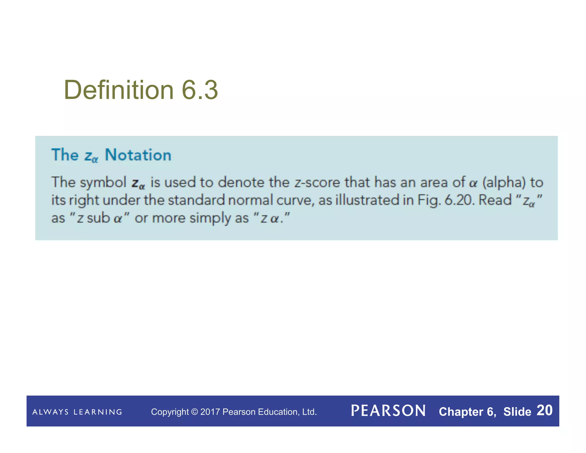
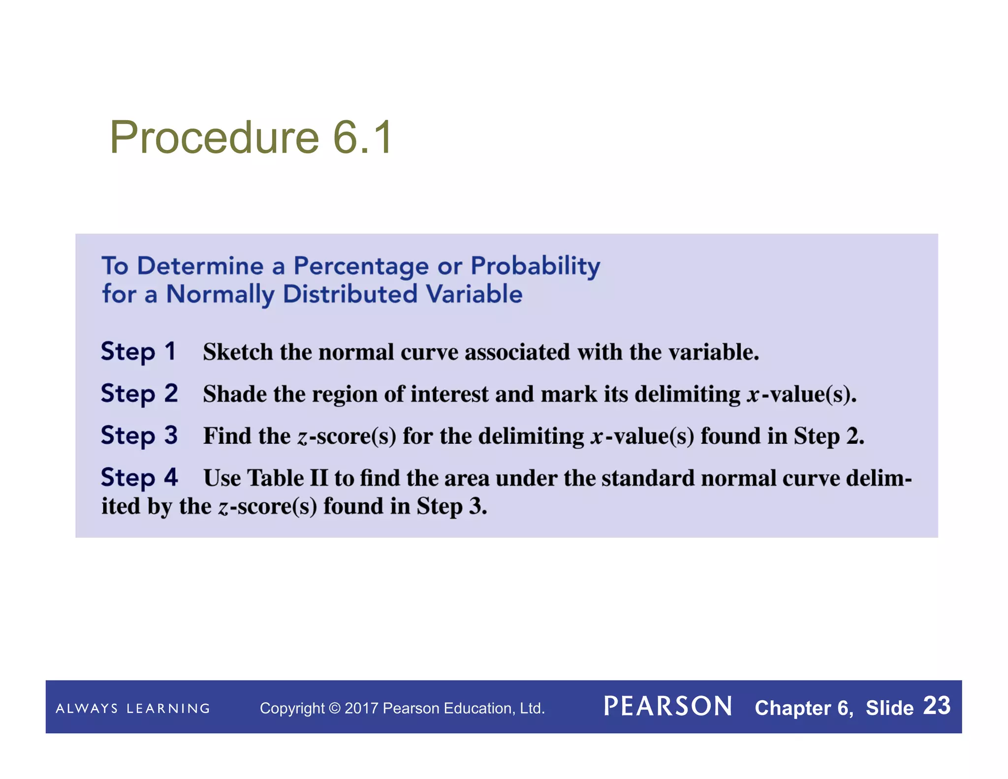
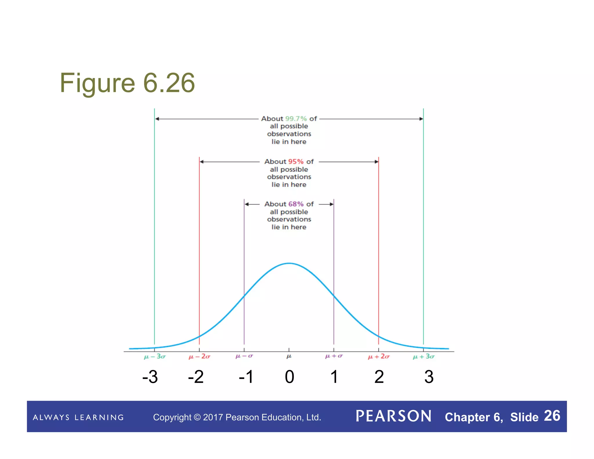
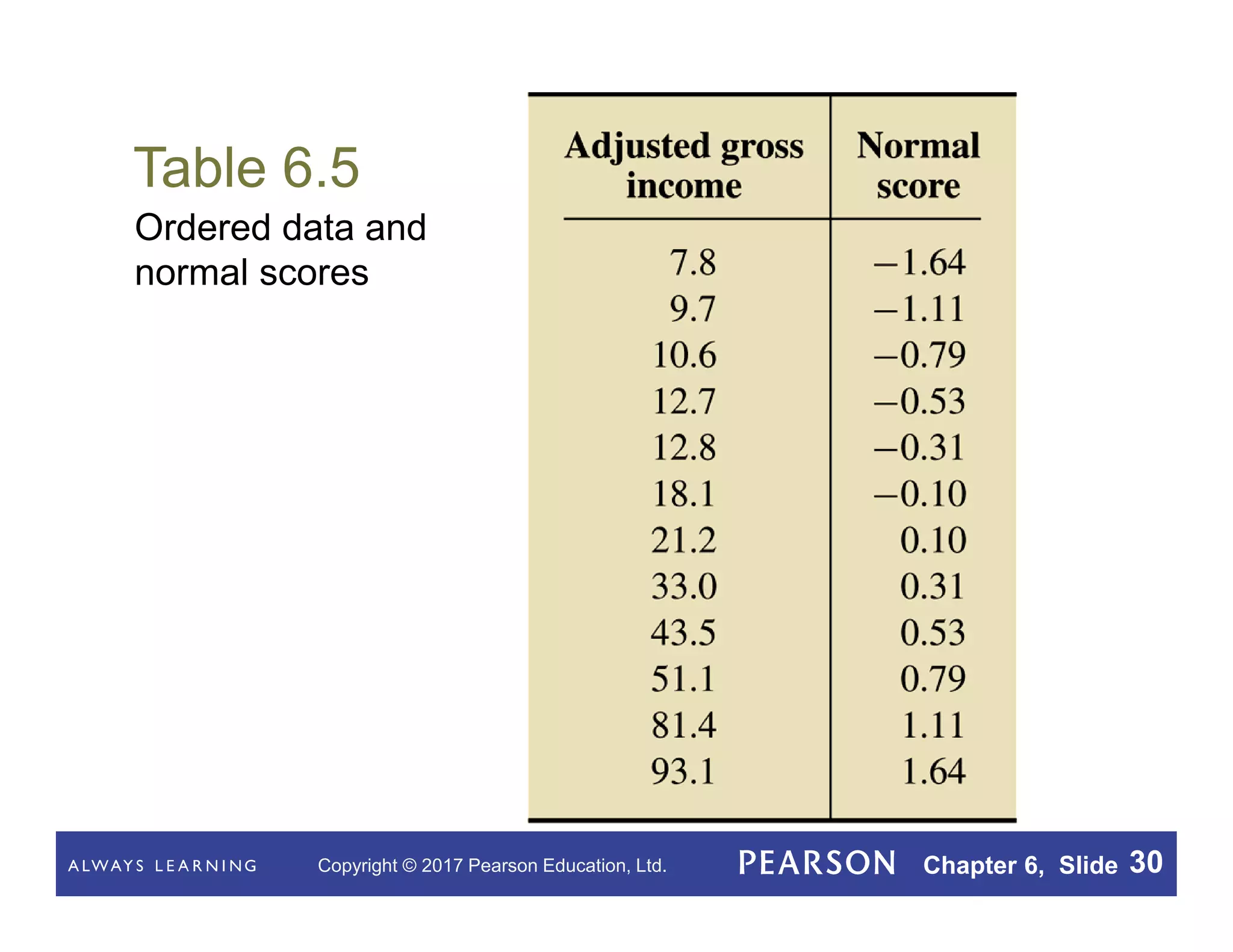
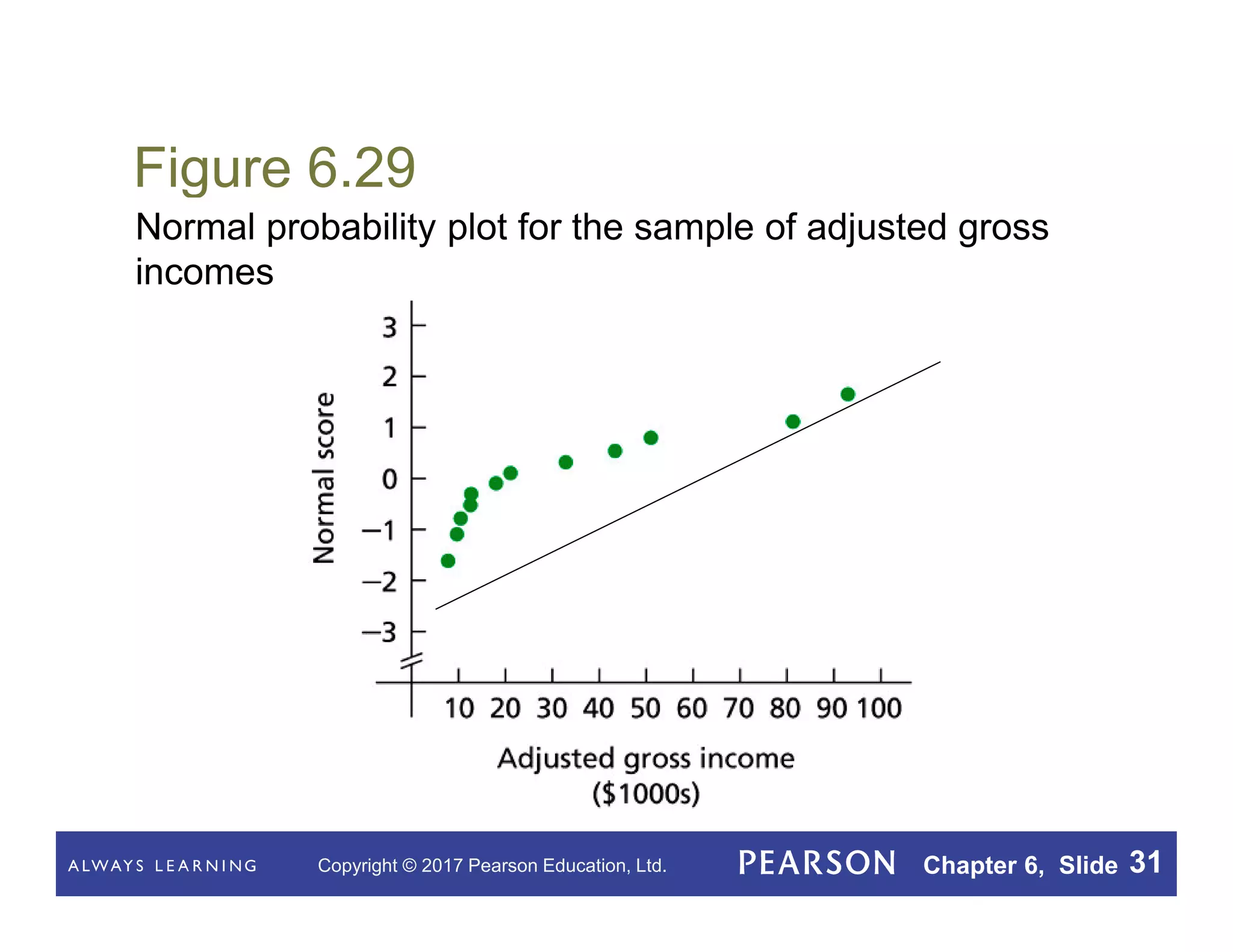
Copyright © 2017 Pearson Education, Ltd. Chapter 6, Slide 1
Chapter 6
The Normal
Distribution

Chapter 6
The Normal Distribution

Section 6.1
Introducing Normally
Distributed Variables

Key Fact 6.1
Basic Properties of Density Curves
Property 1: A density curve is always on or above the
horizontal axis.
Property 2: The total area under a density curve (and
above the horizontal axis) equals 1.

Figure 6.1
Properties 1 and 2 of Key Fact 6.1

Key Fact 6.2
Variables and Their Density Curves
For a variable with a density curve, the percentage of all
possible observations of the variable that lie within any
specified range equals (at least approximately) the
corresponding area under the density curve, expressed
as a percentage.

Figure 6.2
Illustration of Key Fact 6.2

Definition 6.1
Normally Distributed Variable
A variable is said to be a normally distributed variable
or to have a normal distribution if its distribution has the
shape of a normal curve.

Table 6.1
Frequency and relative-frequency
distributions for heights

Figure 6.10 Relative-frequency histogram for
heights with superimposed normal curve

Key Fact 6.3
Normally Distributed Variables and Normal-Curve Areas
For a normally distributed variable, the percentage of all
possible observations that lie within any specified range
equals the corresponding area under its associated normal
curve, expressed as a percentage. This result holds
approximately for a variable that is approximately normally
distributed.

Definition 6.2
Standard Normal Distribution; Standard Normal Curve
A normally distributed variable having mean 0 and
standard deviation 1 is said to have the standard
normal distribution. Its associated normal curve is
called the standard normal curve, which is shown in
Fig. 6.11.
Figure 6.11

Key Fact 6.4

Figure 6.12
Standardizing normal distributions

Figure 6.13
Finding percentages for a normally distributed variable from
areas under the standard normal curve

Section 6.2
Areas Under the Standard
Normal Curve

Key Fact 6.5

Table 6.2
Areas under the standard normal curve

Figure 6.18
Using Table II to find the area under the standard normal
curve that lies (a) to the left of a specified z-score, (b) to
the right of a specified z-score, and (c) between two
specified z-scores
1.23
0.8907
-0.68 1.82
0.2483 0.9656

Definition 6.3

Figures 6.21 & 6.22
Finding z 0.025
Finding z 0.05
Z 0.0344 = -1.82
Zα

Section 6.3
Working with Normally
Distributed Variables

Procedure 6.1

Figure 6.25
Determination of the percentage of people having IQs
between 115 and 140
x=115 x=140
Z1= 115-100/16= 0.94 = 0.8264
Z2= 140-100/16= 2.50 = 0.9938
0.9938-0.8264= 0.1674 16.74%

Key Fact 6.6

Figure 6.26
-3 -2 -1 0 1 2 3

Procedure 6.2

Section 6.4
Assessing Normality; Normal
Probability Plots

Key Fact 6.7

Table 6.5
Ordered data and
normal scores

Figure 6.29
Normal probability plot for the sample of adjusted gross
incomes

Normal Distribution.pdf

More Related Content

What's hot

Similar to Normal Distribution.pdf

More from RAHULSUTHAR46

Recently uploaded

Normal Distribution.pdf