Descriptive measures.pdf

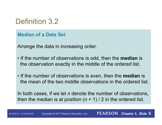
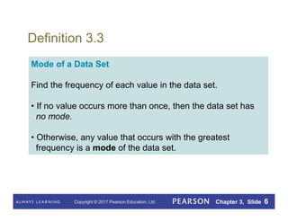
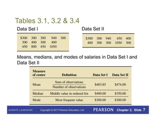
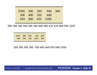
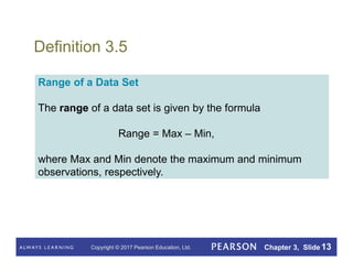
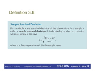
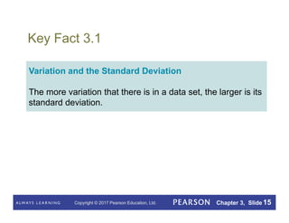
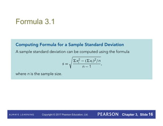
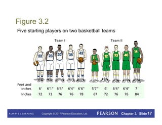
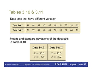
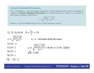
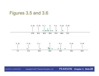
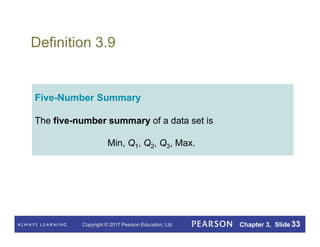
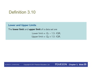
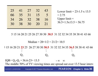
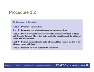
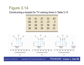
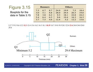
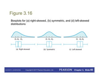
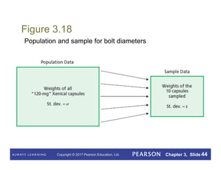
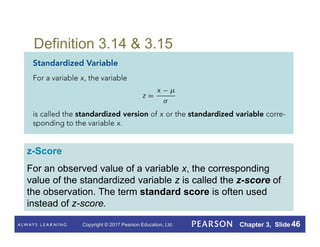
Copyright © 2017 Pearson Education, Ltd. Chapter 3, Slide 1
Chapter 3
Descriptive
Measures

Chapter 3
Descriptive Measures

Section 3.1
Measures of Center

Definition 3.1
Mean of a Data Set
The mean of a data set is the sum of the observations
divided by the number of observations.

Definition 3.2
Median of a Data Set
Arrange the data in increasing order.
• If the number of observations is odd, then the median is
the observation exactly in the middle of the ordered list.
• If the number of observations is even, then the median is
the mean of the two middle observations in the ordered list.
In both cases, if we let n denote the number of observations,
then the median is at position (n + 1) / 2 in the ordered list.

Definition 3.3
Mode of a Data Set
Find the frequency of each value in the data set.
• If no value occurs more than once, then the data set has
no mode.
• Otherwise, any value that occurs with the greatest
frequency is a mode of the data set.

Tables 3.1, 3.2 & 3.4
Data Set I Data Set II
Means, medians, and modes of salaries in Data Set I and
Data Set II

300 300 300 300 300 300 400 400 450 450 800 940 1050
300 300 300 300 300 400 400 450 940 1050

Figure 3.1
Relative positions of the mean and median for
(a) right-skewed, (b) symmetric, and (c) left-skewed
distributions

Definition 3.4

Section 3.2
Measures of Variation

Figure 3.3
Shortest and tallest starting players on the teams

Definition 3.5
Range of a Data Set
The range of a data set is given by the formula
Range = Max – Min,
where Max and Min denote the maximum and minimum
observations, respectively.

Definition 3.6

Key Fact 3.1
Variation and the Standard Deviation
The more variation that there is in a data set, the larger is its
standard deviation.

Formula 3.1

Figure 3.2
Five starting players on two basketball teams

Tables 3.10 & 3.11
Data sets that have different variation
Means and standard deviations of the data sets
in Table 3.10

78 – 75= 3

Figures 3.5 and 3.6

Key Fact 3.2
Three-Standard-Deviations Rule
Almost all the observations in any data set lie within three
standard deviations to either side of the mean.

Section 3.3
Empirical Rule

Key Fact 3.4

Figure 3.9

Table 3.12
PCB concentrations, in parts per million, of 60 pelican eggs

Figure 3.10
Histogram of the PCB-concentration data

Figure 3.10
The mean and one, two, and three standard deviations to either
side of the mean for the PCB-concentration data

Section 3.4
The Five-Number Summary; Boxplots

Percentiles: 100 equal part
Deciles –
quantiles –
quartiles –
divide 10 equal part
divide 5 equal part
divide 4 equal part

Definition 3.7
Quartiles
First, arrange the data in increasing order. Next, determine
the median. Then, divide the (ordered) data set into two
halves, a bottom half and a top half; if the number of
observations is odd, include the median in both halves.
• The first quartile (Q1) is the median of the bottom half of the data set.
• The second quartile (Q2) is the median of the entire data set.
• The third quartile (Q3) is the median of the top half of the data set.

Procedure 3.1

Definition 3.8
Interquartile Range
The interquartile range, or IQR, is the difference between
the first and third quartiles; that is, IQR = Q3 – Q1.

Definition 3.9
Five-Number Summary
The five-number summary of a data set is
Min, Q1, Q2, Q3, Max.

Figure 3.12
Quartiles for (a) uniform, (b) bell-shaped, (c) right-skewed, and
(d) left-skewed distributions
Median – Q2
Third quarter = Q3 – Q 2
First quarter= Q1 – Minimmum
Second quarter= Q 2 - Q1
Four quarter = Max- Q3

Definition 3.10

5 15 16 20 21 23 25 26 27 30 30 30.5 31 32 32 34 35 36.5 38 38 41 43 66
Q2
Q1 Q3
IQR= Q3-Q1 = 36.6-23= 13.5
The middle 50% of TV viewing times are spread out over 13.5 hour intervals.
5 15 16 20 21 25 26 27 30 30 30.5 31 32 32 34 35 38 38 41 43 66
Median = 20+1/2 = 21/2= 10.5
- ∞ ∞
Lower limit = 23-1.5 x 13.5
= 2.75
Upper limit =
36.5+1.5x13.5 = 56.75

Procedure 3.2

Figure 3.14
Constructing a boxplot for TV viewing times in Table 3.13

Figure 3.15
Boxplots for the
data in Table 3.15
Q3
Q1
Q2
29.4 Maximum
Minimum 5.2
5.2 7.5 9.3 9.6 12.2 12.3 12.4 15.6 16.3 16.3 18.1 18.35 18.7 19.0 19.9 20.3 22.8 23.4 24.0 24.0 28.0
29.4

Figure 3.16
Boxplots for (a) right-skewed, (b) symmetric, and (d) left-skewed
distributions

Section 3.5
Descriptive Measures for Populations;
Use of Samples

Definition 3.11

Definition 3.12

Figure 3.18
Population and sample for bolt diameters

Definition 3.13
Parameter and Statistic
Parameter: A descriptive measure for a population.µ
Statistic: A descriptive measure for a sample. x and s

Definition 3.14 & 3.15
z-Score
For an observed value of a variable x, the corresponding
value of the standardized variable z is called the z-score of
the observation. The term standard score is often used
instead of z-score.

Descriptive measures.pdf

More Related Content

Similar to Descriptive measures.pdf

More from RAHULSUTHAR46

Recently uploaded

Descriptive measures.pdf