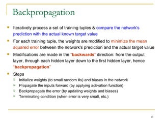
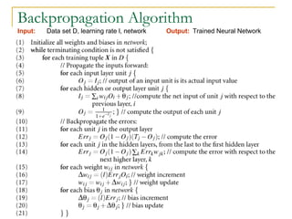
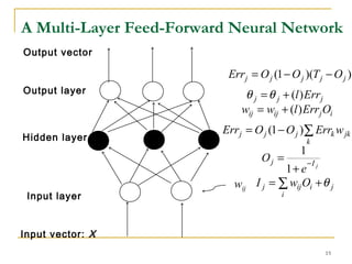
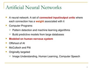
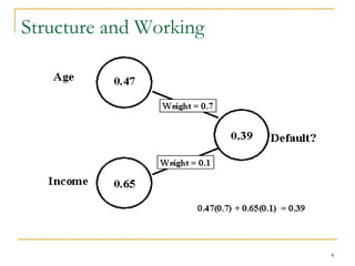
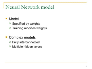
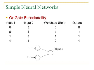
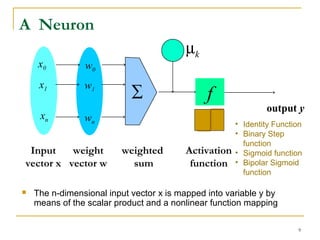
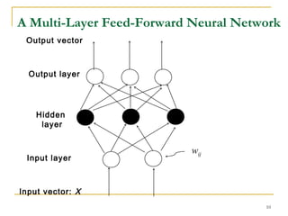
The document discusses artificial neural networks and classification using backpropagation, describing neural networks as sets of connected input and output units where each connection has an associated weight. It explains backpropagation as a neural network learning algorithm that trains networks by adjusting weights to correctly predict the class label of input data, and how multi-layer feed-forward neural networks can be used for classification by propagating inputs through hidden layers to generate outputs.

1. 1
Classification by
Back Propagation

2. Artificial Neural Networks
 A neural network: A set of connected input/output units where
each connection has a weight associated with it
 Computer Programs
 Pattern detection and machine learning algorithms
 Build predictive models from large databases
 Modeled on human nervous system
 Offshoot of AI
 McCulloch and Pitt
 Originally targeted
 Image Understanding, Human Learning, Computer Speech
2

3. Features
 Highly accurate predictive models for a large number of
different types of problems
 Ease of use and deployment – poor
 Connection between nodes
 Number of units
 Training level
 Learning Capability
 Model is built one record at a time
3

4. Structure and Working
4

5. Neural Network model
 Model
 Specified by weights
 Training modifies weights
 Complex models
 Fully interconnected
 Multiple hidden layers
5

6. Simple Neural Networks
 Or Gate Functionality
Input 1 Input 2 Weighted Sum Output
0 0 0 0
0 1 1 1
1 0 1 1
1 1 2 1
6
I1
I2
Output

7. 7
Classification by Backpropagation
 Backpropagation: A neural network learning algorithm
 Started by psychologists and neurobiologists to develop and
test computational analogues of neurons
 During the learning phase, the network learns by adjusting
the weights so as to be able to predict the correct class label
of the input tuples
 Also referred to as connectionist learning due to the
connections between units

8. 8
Neural Network as a Classifier
 Weakness
 Long training time
 Require a number of parameters typically best determined empirically, e.g.,
the network topology or “structure."
 Poor interpretability: Difficult to interpret the symbolic meaning behind the
learned weights and of “hidden units" in the network
 Strength
 High tolerance to noisy data
 Ability to classify untrained patterns
 Well-suited for continuous-valued inputs and outputs
 Successful on a wide array of real-world data
 Algorithms are inherently parallel
 Techniques have recently been developed for the extraction of rules from
trained neural networks

9. 9
A Neuron
 The n-dimensional input vector x is mapped into variable y by
means of the scalar product and a nonlinear function mapping
µk-
f
weighted
sum
Input
vector x
output y
Activation
function
weight
vector w
∑
w0
w1
wn
x0
x1
xn
• Identity Function
• Binary Step
function
• Sigmoid function
• Bipolar Sigmoid
function

10. 10
A Multi-Layer Feed-Forward Neural Network
Output layer
Input layer
Hidden
layer
Output vector
Input vector: X
wij

11. 11
Multi-Layer Neural Network
 The inputs to the network correspond to the attributes measured for
each training tuple
 Inputs are fed simultaneously into the units making up the input layer
 They are then weighted and fed simultaneously to a hidden layer
 The number of hidden layers is arbitrary, although usually only one
 The weighted outputs of the last hidden layer are input to units making
up the output layer, which emits the network's prediction
 The network is feed-forward in that none of the weights cycles back to
an input unit or to an output unit of a previous layer

12. 12
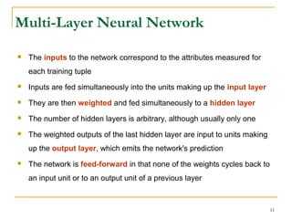
Defining a Network Topology
 First decide the network topology: # of units in the input layer, # of
hidden layers (if > 1), # of units in each hidden layer, and # of units in the
output layer
 Normalizing the input values for each attribute measured in the training
tuples to [0.0—1.0]
 One input unit per domain value, each initialized to 0
 Output, if for classification and more than two classes, one output unit per
class is used
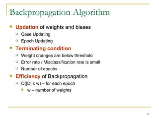
 Once a network has been trained and its accuracy is unacceptable,
repeat the training process with a different network topology or a different
set of initial weights

13. 13
Backpropagation
 Iteratively process a set of training tuples & compare the network's
prediction with the actual known target value
 For each training tuple, the weights are modified to minimize the mean
squared error between the network's prediction and the actual target value
 Modifications are made in the “backwards” direction: from the output
layer, through each hidden layer down to the first hidden layer, hence
“backpropagation”
 Steps
 Initialize weights (to small random #s) and biases in the network
 Propagate the inputs forward (by applying activation function)
 Backpropagate the error (by updating weights and biases)
 Terminating condition (when error is very small, etc.)

14. 14
Backpropagation Algorithm
Input: Data set D, learning rate l, network Output: Trained Neural Network

15. 15
A Multi-Layer Feed-Forward Neural Network
Output layer
Input layer
Hidden layer
Output vector
Input vector: X
wij ∑ +=
i
jiijj OwI θ
jIj
e
O −
+
=
1
1
))(1( jjjjj OTOOErr −−=
jk
k
kjjj wErrOOErr ∑−= )1(
ijijij OErrlww )(+=
jjj Errl)(+=θθ

16. 16
Backpropagation Algorithm
 Updation of weights and biases
 Case Updating
 Epoch Updating
 Terminating condition
 Weight changes are below threshold
 Error rate / Misclassification rate is small
 Number of epochs
 Efficiency of Backpropagation
 O(|D| x w) – for each epoch
 w – number of weights

17. 17
Backpropagation Example

18. 18
Backpropagation Example

19. 19
Backpropagation and Interpretability
 Rule extraction from networks: network pruning
 Simplify the network structure by removing weighted links that have
the least effect on the trained network
 Then perform link, unit, or activation value clustering
 The set of input and activation values are studied to derive rules
describing the relationship between the input and hidden unit layers
 Sensitivity analysis: assess the impact that a given input variable
has on a network output. The knowledge gained from this analysis
can be represented in rules

20. 20
Rules from the network