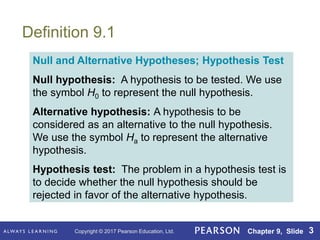
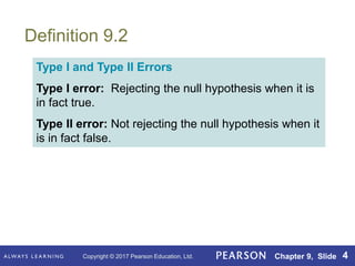
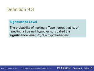
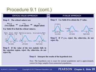
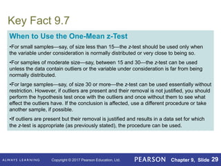
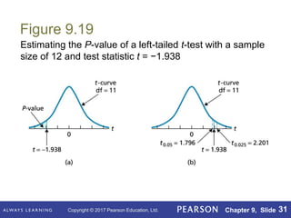
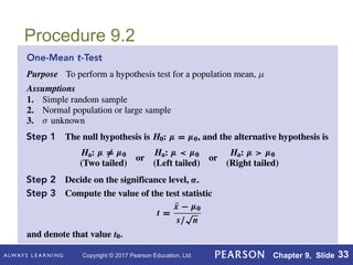
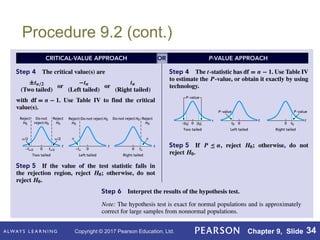
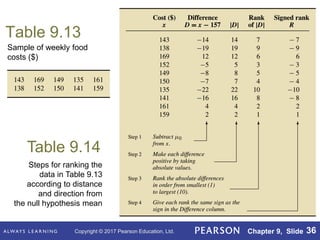
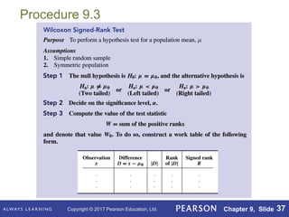
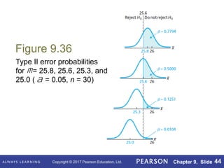
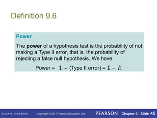
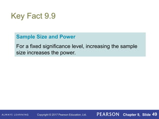
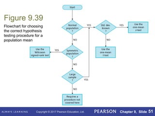
Hypothesis tests for one population mean.pdf

Copyright © 2017 Pearson Education, Ltd. Chapter 9, Slide 1
Chapter 9
Hypothesis Tests
for One Population
Mean

Section 9.1
The Nature of Hypothesis
Testing

Definition 9.1
Null and Alternative Hypotheses; Hypothesis Test
Null hypothesis: A hypothesis to be tested. We use
the symbol H0 to represent the null hypothesis.
Alternative hypothesis: A hypothesis to be
considered as an alternative to the null hypothesis.
We use the symbol Ha to represent the alternative
hypothesis.
Hypothesis test: The problem in a hypothesis test is
to decide whether the null hypothesis should be
rejected in favor of the alternative hypothesis.

Definition 9.2
Type I and Type II Errors
Type I error: Rejecting the null hypothesis when it is
in fact true.
Type II error: Not rejecting the null hypothesis when it
is in fact false.

Definition 9.3
Significance Level
The probability of making a Type I error, that is, of
rejecting a true null hypothesis, is called the
significance level, , of a hypothesis test.
a

Key Fact 9.1

Key Fact 9.2
Possible Conclusions for a Hypothesis Test
Suppose that a hypothesis test is conducted at a small
significance level.
• If the null hypothesis is rejected, we conclude that
the data provide sufficient evidence to support the
alternative hypothesis.
• If the null hypothesis is not rejected, we conclude
that the data do not provide sufficient evidence to
support the alternative hypothesis.

Section 9.2
Critical-Value Approach to
Hypothesis Testing

Figure 9.2
Criterion for deciding whether to reject the null hypothesis

Figure 9.3
Rejection region, nonrejection region, and critical value for
the golf-driving-distances hypothesis test

Definition 9.4
Rejection Region, Nonrejection Region, and Critical
Values
Rejection region: The set of values for the test statistic
that leads to rejection of the null hypothesis.
Nonrejection region: The set of values for the test
statistic that leads to nonrejection of the null hypothesis.
Critical value(s): The value or values of the test
statistic that separate the rejection and nonrejection
regions. A critical value is considered part of the
rejection region.

Figure 9.4
Graphical display of rejection regions for two-tailed, left-
tailed, and right-tailed tests

Definition 9.3

Figure 9.5
Critical value(s) for a one-mean z-test at the significance
level if the test is (a) two tailed, (b) left tailed, or
(c) right tailed
a

Section 9.3
P-Value Approach to
Hypothesis Testing

Figure 9.7
P-value for golf-driving-distances hypothesis test

Definition 9.5
P-Value
The P-value of a hypothesis test is the probability of
getting sample data at least as inconsistent with the
null hypothesis (and supportive of the alternative
hypothesis) as the sample data actually obtained. We
use the letter P to denote the P-value.

Key Fact 9.4

Key Fact 9.5

Key Fact 9.6
Determining a P-Value
To determine the P-value of a hypothesis test, we
assume that the null hypothesis is true and compute
the probability of observing a value of the test statistic
as extreme as or more extreme than that observed.
By extreme we mean “far from what we would expect
to observe if the null hypothesis is true.”

Figure 9.8
P-value for a one-mean z-test if the test is (a) two tailed, (b)
left tailed, or (c) right tailed

Figure 9.9
Value of the test statistic and the P-value

Table 9.7
General steps for the P-value approach to hypothesis
testing

Table 9.8
Guidelines for using the P-value to assess the evidence
against the null hypothesis

Procedure 9.1

Procedure 9.1 (cont.)

Key Fact 9.7
When to Use the One-Mean z-Test
•For small samples—say, of size less than 15—the z-test should be used only when
the variable under consideration is normally distributed or very close to being so.
•For samples of moderate size—say, between 15 and 30—the z-test can be used
unless the data contain outliers or the variable under consideration is far from being
normally distributed.
•For large samples—say, of size 30 or more—the z-test can be used essentially without
restriction. However, if outliers are present and their removal is not justified, you should
perform the hypothesis test once with the outliers and once without them to see what
effect the outliers have. If the conclusion is affected, use a different procedure or take
another sample, if possible.
•If outliers are present but their removal is justified and results in a data set for which
the z-test is appropriate (as previously stated), the procedure can be used.

Figure 9.19
Estimating the P-value of a left-tailed t-test with a sample
size of 12 and test statistic t = −1.938

Figure 9.20
Estimating the P-value of a two-tailed t-test with a sample
size of 25 and test statistic t =−0.895

Procedure 9.2

Section 9.6
The Wilcoxon Signed-Rank Test

Table 9.13
Steps for ranking the
data in Table 9.13
according to distance
and direction from
the null hypothesis mean
Table 9.14
Sample of weekly food
costs ($)

Procedure 9.3

Key Fact 9.8
Wilcoxon Signed-Rank Test Versus the t-Test
Suppose that you want to perform a hypothesis test for a population
mean. When deciding between the t-test and the Wilcoxon signed-rank
test, follow these guidelines:
• If you are reasonably sure that the variable under consideration is
normally distributed, use the t-test.
• If you are not reasonably sure that the variable under consideration
is normally distributed but are reasonably sure that it has a
symmetric distribution, use the Wilcoxon signed-rank test.

Section 9.7
Type II Error Probabilities;
Power

Figure 9.30
Decision criterion for the gas mileage illustration
(α = 0.05, n = 30)

Figure 9.31
Determining the probability of a Type II error if = 25.8 mpg
m

Procedure 9.4

Figure 9.36
Type II error probabilities
for = 25.8, 25.6, 25.3, and
25.0 ( = 0.05, n = 30)
m
a

Definition 9.6
Power
The power of a hypothesis test is the probability of not
making a Type II error, that is, the probability of
rejecting a false null hypothesis. We have
Power = (Type II error) = .
1 - 1 - b

Procedure 9.5

Figure 9.38
Power curves for the gas mileage illustration when n = 30
and n = 100 ( = 0.05)
a

Key Fact 9.9
Sample Size and Power
For a fixed significance level, increasing the sample
size increases the power.

Section 9.8
Which Procedure Should Be Used?

Flowchart for choosing
the correct hypothesis
testing procedure for a
population mean
Figure 9.39

Hypothesis tests for one population mean.pdf

More Related Content

What's hot

Similar to Hypothesis tests for one population mean.pdf

More from RAHULSUTHAR46

Recently uploaded

Hypothesis tests for one population mean.pdf