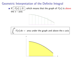
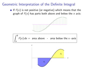
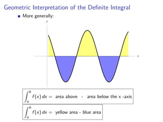
Riemann Sums
     Consider any function f (x) where a ≤ x ≤ b.
                                                                                        b−a
     Partition [a, b] into n subintervals of equal length ∆x =
                                                                                         n
     Evaluate the function f (x) at sample points c1 , c2 , ... cn
     chosen inside each subinterval.
              Y

                                            Positive values


               a        x0   x1        x2         x3           x4        x5    b   x6
                   c1             c2        c3            c4        c5        c6
                                                                                   X


                                                 Negative values


     Form the Riemann sum:
                  f (c1 ) · ∆x + f (c2 ) · ∆x + ... + f (cn ) · ∆x
Riemann Sum: [f (c1 ) + f (c2 ) + ... + f (cn )] · ∆x

        Y


                                 Positive values


        a    x0   x1        x2           x3                   x4        x5    b   x6
            c1                    c3                     c4        c5        c6
    O                  c2                                                              X


                                       Negative values
The Definite Integral
      Notation:
                                                               n
      f (c1 ) · ∆x + f (c2 ) · ∆x + ... + f (cn ) · ∆x =            f (ci ) · ∆x
                                                              i=1
      Consider more and more subintervals. In other words, let the
      number n be larger and larger:
                  Y


                                                                       X


      Then the limit of the Riemann sums, as the number of
      intervals becomes larger and larger is called The Definite
      Integral or The Riemann Integral of f (x) from a to b:
                            b                     n
                                f (x) dx = lim         f (ci ) ∆x
                        a                 n→∞
                                                 i=1
Geometric Interpretation of the Definite Integral
       If f (x) ≥ 0 , which means that the graph of f (x) is above
       the x - axis:


             b
                 f (x) dx = area under the graph and above the x axis
         a
                           y


                                                         x
Geometric Interpretation of the Definite Integral
       If f (x) is not positive (or negative) which means that the
       graph of f (x) has parts both above and below the x axis:


             b
                 f (x) dx = area above - area below the x -axis
         a
                           y


                                                  A1

                                                        x

                                    A2
Geometric Interpretation of the Definite Integral
       More generally:
                        y


                                                                  x


             b
                 f (x) dx = area above - area below the x -axis
         a
             b
                 f (x) dx = yellow area - blue area
         a

The Definite Integral

  • 1.
    Riemann Sums Consider any function f (x) where a ≤ x ≤ b. b−a Partition [a, b] into n subintervals of equal length ∆x = n Evaluate the function f (x) at sample points c1 , c2 , ... cn chosen inside each subinterval. Y Positive values a x0 x1 x2 x3 x4 x5 b x6 c1 c2 c3 c4 c5 c6 X Negative values Form the Riemann sum: f (c1 ) · ∆x + f (c2 ) · ∆x + ... + f (cn ) · ∆x
  • 2.
    Riemann Sum: [f(c1 ) + f (c2 ) + ... + f (cn )] · ∆x Y Positive values a x0 x1 x2 x3 x4 x5 b x6 c1 c3 c4 c5 c6 O c2 X Negative values
  • 3.
    The Definite Integral Notation: n f (c1 ) · ∆x + f (c2 ) · ∆x + ... + f (cn ) · ∆x = f (ci ) · ∆x i=1 Consider more and more subintervals. In other words, let the number n be larger and larger: Y X Then the limit of the Riemann sums, as the number of intervals becomes larger and larger is called The Definite Integral or The Riemann Integral of f (x) from a to b: b n f (x) dx = lim f (ci ) ∆x a n→∞ i=1
  • 4.
    Geometric Interpretation ofthe Definite Integral If f (x) ≥ 0 , which means that the graph of f (x) is above the x - axis: b f (x) dx = area under the graph and above the x axis a y x
  • 5.
    Geometric Interpretation ofthe Definite Integral If f (x) is not positive (or negative) which means that the graph of f (x) has parts both above and below the x axis: b f (x) dx = area above - area below the x -axis a y A1 x A2
  • 6.
    Geometric Interpretation ofthe Definite Integral More generally: y x b f (x) dx = area above - area below the x -axis a b f (x) dx = yellow area - blue area a