This document provides an overview of linear models for classification. It discusses discriminant functions including linear discriminant analysis and the perceptron algorithm. It also covers probabilistic generative models that model class-conditional densities and priors to estimate posterior probabilities. Probabilistic discriminative models like logistic regression directly model posterior probabilities using maximum likelihood. Iterative reweighted least squares is used to optimize logistic regression since there is no closed-form solution.


![Linear Models for Classification
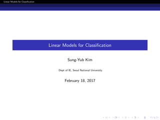
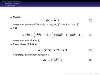
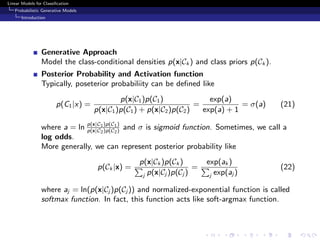
Probabilistic Generative Models
MLE
Gaussian clas-conditional density
Likelihood function is
p(t, X|π, µ1, µ2, Σ) =
N
n=1
[πN(xn|µ1, Σ)]tn
[(1 − π)N(xn|µ2, Σ)]1−tn
(26)
where π is class prior probability, µk is class-mean, tn is 1 if class of n-th
data is 1, otherwise 0 and we assume that classes share covariance.
Closed-form Solution
We can solve this problem exactly
π =
N1
N1 + N2
(27)
µ1 =
1
N1
N
n=1
tnxn, µ2 =
1
N2
N
n=1
(1 − tn)xn (28)
S =
N1
N
S1 +
N2
N
S2 (29)
where
S1 = 1
N1 n∈C1
(xn − µ1)(xn − µ1)T
andS2 = 1
N2 n∈C2
(xn − µ2)(xn − µ2)T](https://image.slidesharecdn.com/linearmodelsforclassification-170218134122/85/Linear-models-for-classification-14-320.jpg)


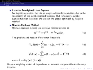
![Linear Models for Classification
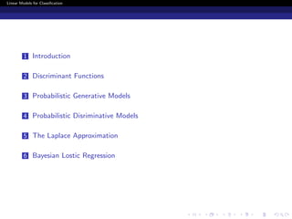
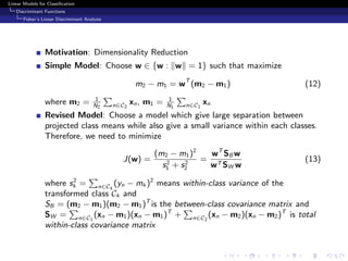
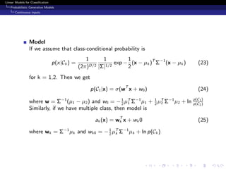
Probabilistic Disriminative Models
Logistic Regression
Model
p(C1|φ) = y(φ) = σ(wT
φ) (35)
If we use this model, we just need to find M adaptive parameters. It is
relatively simpler than Gaussian model which is need to be find its
covariance paramters.
Likelihood
We can write likelihood as
p(t|w) =
N
n=1
ytn
n {1 − yn}1−tn
(36)
and we can use this likelihood function to make cross entropy error
function like
E(w) = Et [− ln y] −
N
n=1
{tn ln yn + (1 − tn) ln(1 − yn)} (37)](https://image.slidesharecdn.com/linearmodelsforclassification-170218134122/85/Linear-models-for-classification-18-320.jpg)
![Linear Models for Classification
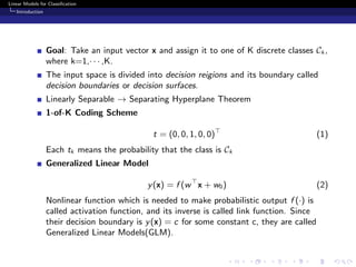
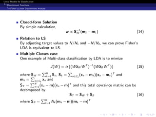
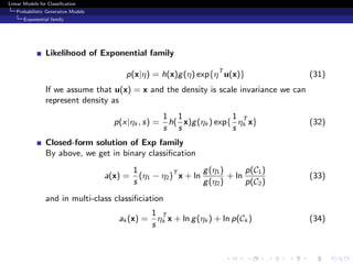
Probabilistic Disriminative Models
Multiclass Logistic Regression
Likelihood
Similar in binary case, we can get likelihood of our model
p(T|w1, . . . , wK ) =
N
n=1
K
k=1
y
tnk
nk (44)
Take negaitve logarithm to get cross entropy error function
E(w1, . . . , wK ) = ET[− ln p(y)] −
N
n=1
K
k=1
tnk ln ynk (45)
By similar argument in binary case, we can get
wj E(w1, . . . , wK ) =
N
n=1
(ynj − tnj )φn (46)
wk wj E(w1, . . . , wK ) =
N
n=1
ynk (Ikj − ynj )φnφT
n (47)](https://image.slidesharecdn.com/linearmodelsforclassification-170218134122/85/Linear-models-for-classification-21-320.jpg)
![Linear Models for Classification
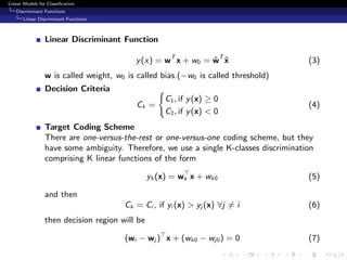
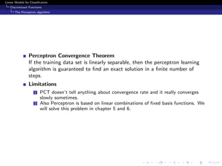
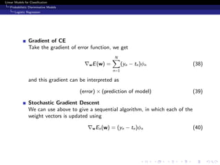
Probabilistic Disriminative Models
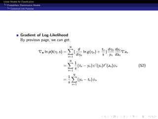
Canonical Link Functios
Canonical Link Function
Assuming a conditional distribution for the target variable from the
exponential family, along with a corresponding choice for the activation
function known as the canonical link function.
Likelihood function First we assume scale invariant exponential
class-conditional distribution
p(t|η, s) =
1
s
h(
t
s
)g(η) exp{
ηt
s
} (49)
By definition of 1st statistics, we get
y = E[t|η] = −s
d
dη
ln g(η) (50)
WLOG we denote this relation as η = ψ(y). In the definition of GLM, we
call f (·) activation function. We call inverse of this function, f −1
(·), link
function. Meanwhile log-likelihood function is
ln p(t|η, s) =
N
n=1
{ln g(ηn) +
ηntn
s
} + const. (51)](https://image.slidesharecdn.com/linearmodelsforclassification-170218134122/85/Linear-models-for-classification-23-320.jpg)

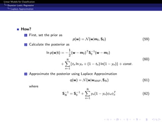
![Linear Models for Classification
Bayesian Lostic Regression
Predictive Distribution
Predictive Distribution by Laplace Approximation
By using Laplace Approximation, we get
p(C1|φ, t) = p(C1|φ, w)p(w|t)dw σ(wT
φ)q(w)dw (63)
Denoting a = wT
φ we get
σ(wT
φ) = δ(a − wT
φ)σ(a)da (64)
Therefore we get
p(C1|φ, t) σ(a) δ(a − wT
φ)q(w)dwda = σ(a)p(a)da (65)
Since p(a) means marginalize of q(w), we know that p(a) is also Gaussian.
And mean and variance of Gaussian is
µa = E[a] = ap(a)da = wT
φq(w)dw = wT
MAP φ (66)
σ2
a = {a2
E[a]2
}p(a)da = {(wT
φ)2
− (mT
N φ)2
}dwq(w) = φT
SN φ
(67)](https://image.slidesharecdn.com/linearmodelsforclassification-170218134122/85/Linear-models-for-classification-28-320.jpg)


![[DSC Europe 25] Slobodan Dolinic - Smart and Intelligent Green Region.pptx](https://cdn.slidesharecdn.com/ss_thumbnails/0bribinjsp6ghwtvsvor-2-sigre-slobodan-dolinic-260115093812-c9c10e90-thumbnail.jpg?width=640&height=640&fit=bounds)


