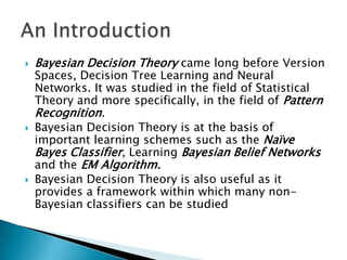
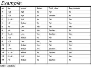
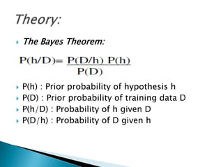
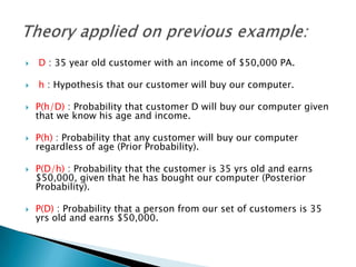
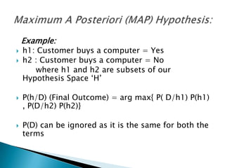
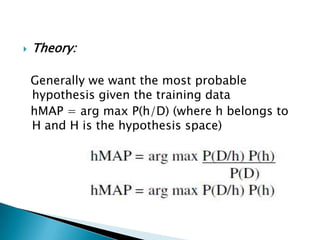
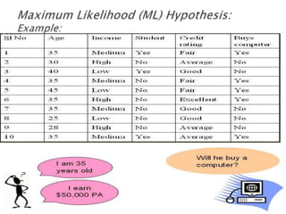
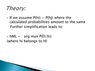
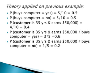
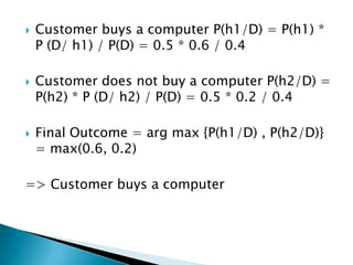
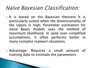
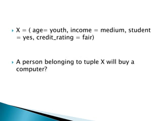
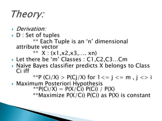
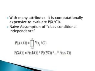
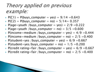
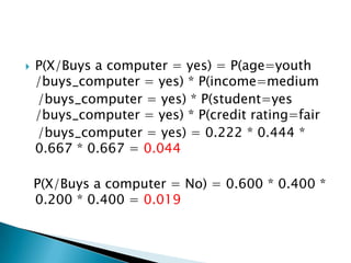
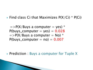
The document provides an overview of Bayesian decision theory and naive Bayesian classification. It discusses how Bayesian decision theory predates other machine learning techniques and forms the basis of classifiers like naive Bayes. It then explains the Bayes theorem and how it is used for probability inference and decision making. An example of predicting whether a customer will buy a computer is used to illustrate Bayesian reasoning. Finally, the document describes how the naive Bayes classifier works by making a strong independence assumption between features to simplify computations. It gives the mathematical formulas and works through an example to classify a customer profile.

1. MUSA AL-HAWAMDAH
128129001011

2.  Bayesian Decision Theory came long before Version
Spaces, Decision Tree Learning and Neural
Networks. It was studied in the field of Statistical
Theory and more specifically, in the field of Pattern
Recognition.
 Bayesian Decision Theory is at the basis of
important learning schemes such as the Naïve
Bayes Classifier, Learning Bayesian Belief Networks
and the EM Algorithm.
 Bayesian Decision Theory is also useful as it
provides a framework within which many non-
Bayesian classifiers can be studied

3.  Bayesian reasoning is applied to decision
making and inferential statistics that deals
with probability inference. It is used the
knowledge of prior events to predict future
events.
 Example: Predicting the color of marbles in a
baske.t

6.  The Bayes Theorem:
 P(h) : Prior probability of hypothesis h
 P(D) : Prior probability of training data D
 P(h/D) : Probability of h given D
 P(D/h) : Probability of D given h

7.  D : 35 year old customer with an income of $50,000 PA.
 h : Hypothesis that our customer will buy our computer.
 P(h/D) : Probability that customer D will buy our computer given
that we know his age and income.
 P(h) : Probability that any customer will buy our computer
regardless of age (Prior Probability).
 P(D/h) : Probability that the customer is 35 yrs old and earns
$50,000, given that he has bought our computer (Posterior
Probability).
 P(D) : Probability that a person from our set of customers is 35
yrs old and earns $50,000.

8. Example:
 h1: Customer buys a computer = Yes
 h2 : Customer buys a computer = No
where h1 and h2 are subsets of our
Hypothesis Space „H‟
 P(h/D) (Final Outcome) = arg max{ P( D/h1) P(h1)
, P(D/h2) P(h2)}
 P(D) can be ignored as it is the same for both the
terms

9.  Theory:
Generally we want the most probable
hypothesis given the training data
hMAP = arg max P(h/D) (where h belongs to
H and H is the hypothesis space)

11.  If we assume P(hi) = P(hj) where the
calculated probabilities amount to the same
Further simplification leads to:
 hML = arg max P(D/hi)
(where hi belongs to H)

12.  P (buys computer = yes) = 5/10 = 0.5
 P (buys computer = no) = 5/10 = 0.5
 P (customer is 35 yrs & earns $50,000) =
4/10 = 0.4
 P (customer is 35 yrs & earns $50,000 / buys
computer = yes) = 3/5 =0.6
 P (customer is 35 yrs & earns $50,000 / buys
computer = no) = 1/5 = 0.2

13.  Customer buys a computer P(h1/D) = P(h1) *
P (D/ h1) / P(D) = 0.5 * 0.6 / 0.4
 Customer does not buy a computer P(h2/D) =
P(h2) * P (D/ h2) / P(D) = 0.5 * 0.2 / 0.4
 Final Outcome = arg max {P(h1/D) , P(h2/D)}
= max(0.6, 0.2)
=> Customer buys a computer

14. Naïve Bayesian
Classification

15.  It is based on the Bayesian theorem It is
particularly suited when the dimensionality of
the inputs is high. Parameter estimation for
naive Bayes models uses the method of
maximum likelihood. In spite over-simplified
assumptions, it often performs better in
many complex realworl situations.
 Advantage: Requires a small amount of
training data to estimate the parameters

17.  X = ( age= youth, income = medium, student
= yes, credit_rating = fair)
 A person belonging to tuple X will buy a
computer?

18.  Derivation:
 D : Set of tuples
** Each Tuple is an „n‟ dimensional
attribute vector
** X : (x1,x2,x3,…. xn)
 Let there be „m‟ Classes : C1,C2,C3…Cm
 Naïve Bayes classifier predicts X belongs to Class
Ci iff
**P (Ci/X) > P(Cj/X) for 1<= j <= m , j <> i
 Maximum Posteriori Hypothesis
**P(Ci/X) = P(X/Ci) P(Ci) / P(X)
**Maximize P(X/Ci) P(Ci) as P(X) is constant

19.  With many attributes, it is computationally
expensive to evaluate P(X/Ci).
 Naïve Assumption of “class conditional
independence”

20.  P(C1) = P(buys_computer = yes) = 9/14 =0.643
 P(C2) = P(buys_computer = no) = 5/14= 0.357
 P(age=youth /buys_computer = yes) = 2/9 =0.222
 P(age=youth /buys_computer = no) = 3/5 =0.600
 P(income=medium /buys_computer = yes) = 4/9 =0.444
 P(income=medium /buys_computer = no) = 2/5 =0.400
 P(student=yes /buys_computer = yes) = 6/9 =0.667
 P(student=yes/buys_computer = no) = 1/5 =0.200
 P(credit rating=fair /buys_computer = yes) = 6/9 =0.667
 P(credit rating=fair /buys_computer = no) = 2/5 =0.400

21.  P(X/Buys a computer = yes) = P(age=youth
/buys_computer = yes) * P(income=medium
/buys_computer = yes) * P(student=yes
/buys_computer = yes) * P(credit rating=fair
/buys_computer = yes) = 0.222 * 0.444 *
0.667 * 0.667 = 0.044
P(X/Buys a computer = No) = 0.600 * 0.400 *
0.200 * 0.400 = 0.019

22.  Find class Ci that Maximizes P(X/Ci) * P(Ci)
=>P(X/Buys a computer = yes) *
P(buys_computer = yes) = 0.028
=>P(X/Buys a computer = No) *
P(buys_computer = no) = 0.007
 Prediction : Buys a computer for Tuple X

23.  http://en.wikipedia.org/wiki/Bayesian_probability
 http://en.wikipedia.org/wiki/Naive_Bayes_classifier
 http://www.let.rug.nl/~tiedeman/ml05/03_bayesian_hando ut. pdf
 http://www.statsoft.com/textbook/stnaiveb.html
 http://www.cs.cmu.edu/afs/cs.cmu.edu/project/theo-2/www/mlbook/ch6.pdf
 Chai, K.; H. T. Hn, H. L. Chieu; “Bayesian Online Classifiers for Text Classification
and Filtering”,
 Proceedings of the 25th annual international ACM SIGIR conference on Research and
Development in Information Retrieval, August 2002, pp 97-104.
 DATA MINING Concepts and Techniques,Jiawei Han, Micheline Kamber Morgan
Kaufman Publishers, 2003.

24. Thank you